of Netflix shows:

netflix %>%
  count(year = year(date_added), type) %>%
  ggplot(aes(year, n, color = type)) +
  geom_line(size = 1) +
  geom_point() +
  labs(x = NULL,
       y = "# of shows",
       color = NULL,
       title = "# of Shows Added by Netflix") +
  scale_x_continuous(breaks = seq(2008, 2020, 2))

Show duration:

netflix %>%
  filter(!is.na(date_added)) %>%
  ggplot(aes(factor(year(date_added)), duration, fill = type, color = type)) +
  geom_boxplot(alpha = 0.6) +
  facet_wrap(~type, ncol = 1, scales = "free_y") +
  labs(x = NULL,
       y = "minutes/seasons",
       color = NULL,
       fill = NULL,
       title = "How long does movie/tv show last?")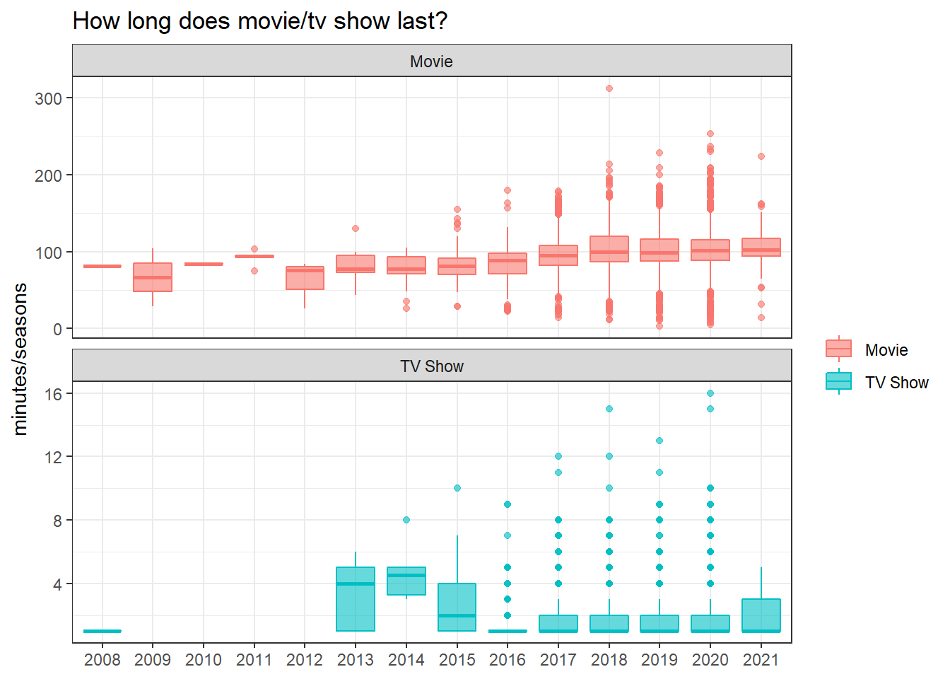 

Weighted log odds on show category per country:

netflix %>%
  separate_rows(category, sep = ", ") %>% 
  count(country, category, sort = T) %>%
  bind_log_odds(country, category, n) %>%
  group_by(country = fct_lump(country, n = 10)) %>%
  slice_max(abs(log_odds_weighted), n = 5, with_ties = F) %>%
  ungroup() %>%
  filter(country != "Other") %>%
  mutate(category = reorder_within(category, log_odds_weighted, country)) %>%
  ggplot(aes(log_odds_weighted, category, fill = country)) +
  geom_col(show.legend = F) +
  facet_wrap(~country, scales = "free_y", ncol = 2) +
  scale_y_reordered() +
  labs(x = "weighted log odds",
       y = NULL,
       title = "Which show category is most characteristic to country?")

How correlated are the categories?

set.seed(2022)

netflix %>%
  separate_rows(category, sep = ", ") %>% 
  pairwise_cor(category, show_id, sort = T) %>%
  head(200) %>%
  ggraph(layout = "fr") +
  geom_edge_link(aes(color = correlation)) +
  geom_node_point() +
  geom_node_text(aes(label = name, color = name), repel = T) +
  scale_edge_color_continuous(low = "pink",
                              high = "green") +
  theme_void() +
  guides(color = "none") +
  labs(edge_width = "correlation",
       title = "How are the categories correlated across shows?") +
  theme(plot.title = element_text(size = 18))

added year - released year:

netflix %>%
  mutate(gap_year = year(date_added) - release_year) %>%
  filter(fct_lump(country, n = 9) != "Other",
         gap_year > 0) %>%
  ggplot(aes(gap_year, fill = type)) +
  geom_histogram(alpha = 0.8) +
  facet_wrap(~country) +
  labs(x = "added year - released year",
       fill = NULL,
       title = "How long does Netflix add shows after their release?") 

netflix %>%
  select(show_id, type, description) %>%
  unnest_tokens(word, description) %>%
  anti_join(stop_words) %>%
  add_count(type, word, name = "type_word_count") %>%
  add_count(word, name = "word_count") %>%
  select(-show_id) %>%
  pivot_longer(cols = c(type_word_count: word_count)) %>%
  distinct() %>%
  filter(name != "word_count") %>%
  group_by(type) %>%
  slice_max(value, n = 20) %>%
  ungroup() %>%
  mutate(word = reorder_within(word, value, type)) %>%
  ggplot(aes(value, word, fill = type)) +
  geom_col(show.legend = F) +
  scale_y_reordered() +
  facet_wrap(~type, scales = "free_y") +
  labs(x = "word frequency",
       y = NULL,
       title = "Top 20 Most Frequent Words in Movies and TV shows")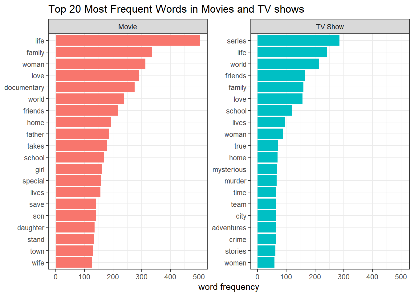

The following idea using pairwise_cor() on type and title is inspired by David Robinson’s code (link).

netflix %>%
  unnest_tokens(word, description) %>%
  anti_join(stop_words, by = "word") %>%
  distinct(type, title, word) %>%
  add_count(word, name = "word_total") %>%
  filter(word_total >= 40) %>%
  pairwise_cor(word, title, sort = TRUE) %>%
  filter(correlation > 0.1) %>%
  ggraph(layout = "fr") +
  geom_edge_link(aes(color = correlation)) +
  geom_node_point() +
  geom_node_text(aes(label = name, color = name), repel = T) +
  scale_edge_color_continuous(low = "pink",
                              high = "green") +
  theme_void() +
  guides(color = "none") +
  labs(edge_width = "correlation",
       title = "How are the description words correlated across shows?") +
  theme(plot.title = element_text(size = 18))

LASSO prediction on if the show has mature contents with the reference:

other_features <- netflix %>%
  select(title, director, cast, category, country) %>%
  pivot_longer(cols = -title, names_to = "feature_type", values_to = "feature") %>%
  filter(!is.na(feature)) %>%
  separate_rows(feature, sep = ", ") %>%
  mutate(feature_type = str_to_title(feature_type)) %>%
  unite(feature, feature_type, feature, sep = ": ") %>%
  add_count(feature, name = "feature_count") %>%
  filter(feature_count >= 10)


feature_matrix <- netflix %>%
  unnest_tokens(word, description) %>%
  anti_join(stop_words, by = "word") %>%
  filter(!is.na(rating)) %>%
  add_count(word, name = "word_total") %>%
  filter(word_total >= 30) %>%
  mutate(feature = paste("Description:", word)) %>%
  bind_rows(other_features) %>% 
  cast_sparse(title, feature)

y <- netflix$mature[match(rownames(feature_matrix), netflix$title)]

# LASSO model
lass_model <- cv.glmnet(feature_matrix, y, family = "binomial") 

lass_model %>%
  .$glmnet.fit %>%
  tidy() %>%
  filter(term != "(Intercept)",
         lambda == lass_model$lambda.1se) %>%
  slice_max(abs(estimate), n = 50) %>%
  mutate(term = fct_reorder(term, estimate)) %>%
  ggplot(aes(estimate, term, fill = estimate > 0)) +
  geom_col() +
  labs(x = NULL,
       y = NULL,
       title = "What feature would contribute the show maturity") +
  theme(legend.position = "none")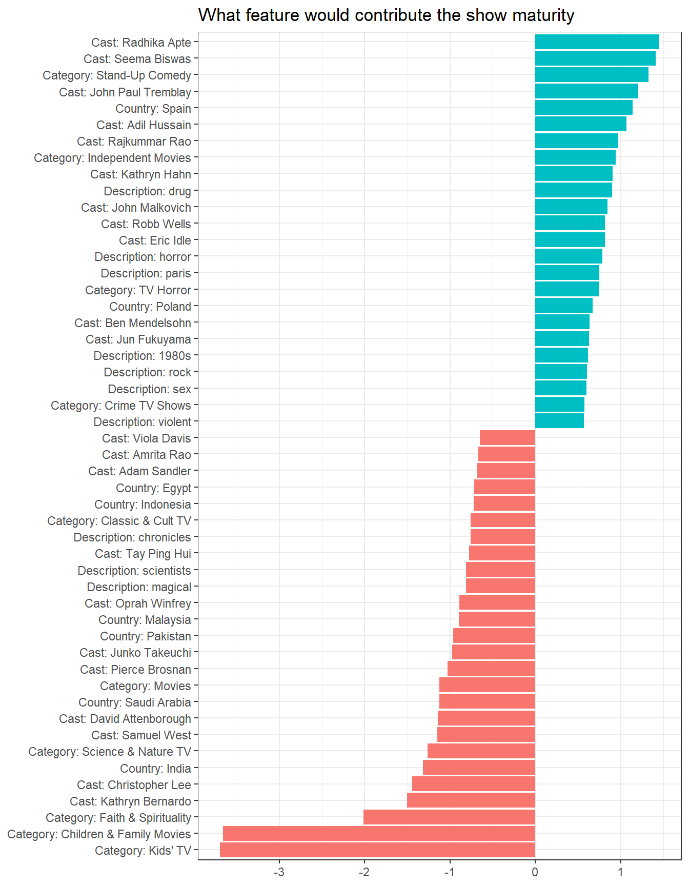 

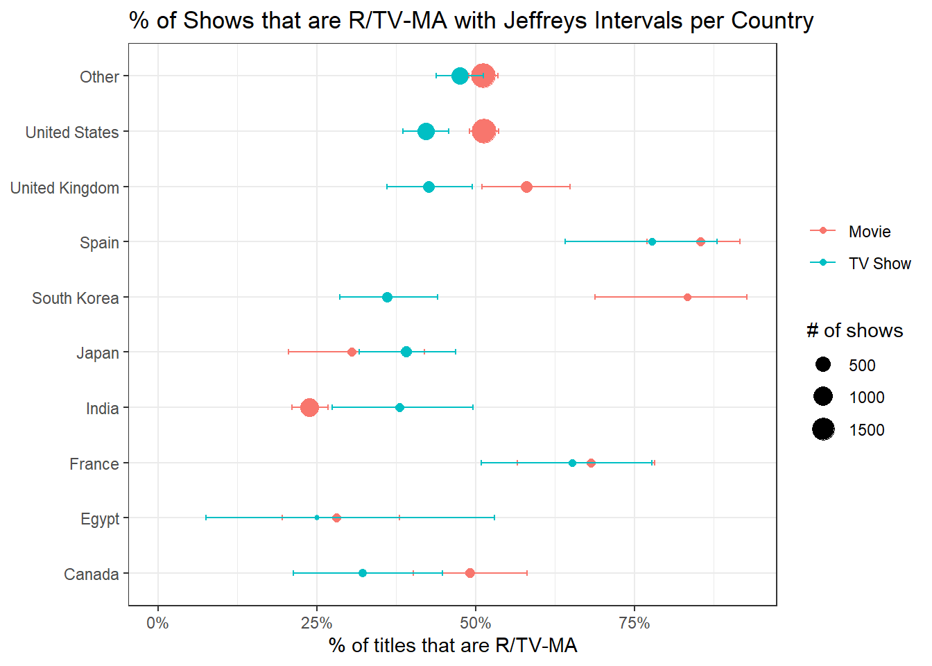
Jeffreys Interval

The following code is largely copied from David Robinson’s code with slight modification (link) for the purposes of learning Jeffreys Interval.

netflix %>%
  filter(!is.na(rating), !is.na(country)) %>%
  group_by(type, country = fct_lump(country, 9)) %>%
  summarize(n_mature = sum(rating %in% c("R", "TV-MA", "NC-17")),
            n = n(),
            .groups = "drop") %>%
  mutate(pct_mature = n_mature / n,
         conf_low = qbeta(.025, n_mature + .5, n - n_mature + .5),
         conf_high = qbeta(.975, n_mature + .5, n - n_mature + .5)) %>%
  ggplot(aes(pct_mature, country, color = type)) +
  geom_point(aes(size = n)) +
  geom_errorbar(aes(xmin = conf_low, xmax = conf_high), width = .1) +
  scale_x_continuous(labels = scales::percent) +
  expand_limits(x = 0) +
  labs(x = "% of titles that are R/TV-MA",
       y = NULL,
       size = "# of shows",
       color = NULL,
       title = "% of Shows that are R/TV-MA with Jeffreys Intervals per Country")