Map Visualization & Tidymodels Practice on Water Resources
This blog post will analyze water resources in Africa. This is an interesting post, because it makes maps by using the ggmap package, and also it exposes some potential problems the tidymodels package has, especially when data has missing values.
library(tidyverse)
library(lubridate)
library(tidymodels)
library(widyr)
library(ggthemes)
library(ggmap)
library(countrycode)
theme_set(theme_bw())
water <- read_csv('https://raw.githubusercontent.com/rfordatascience/tidytuesday/master/data/2021/2021-05-04/water.csv') %>%
mutate(report_date = mdy(report_date)) %>%
rename_with(., ~str_remove(.x, "_deg$")) %>%
rename(country = country_name) %>%
filter(status_id != "u",
lon > -30,
lon < 60,
lat > -50,
lat < 50) %>%
mutate(status_id = if_else(status_id == "y", "has water", "no water"))
water ## # A tibble: 441,214 x 13
## row_id lat lon report_date status_id water_source water_tech
## <dbl> <dbl> <dbl> <date> <chr> <chr> <chr>
## 1 3957 8.07 38.6 2017-04-06 has water <NA> <NA>
## 2 33512 7.37 40.5 2020-08-04 has water Protected Spring <NA>
## 3 35125 0.773 34.9 2015-03-18 has water Protected Shallow Well <NA>
## 4 37760 0.781 35.0 2015-03-18 has water Borehole <NA>
## 5 38118 0.779 35.0 2015-03-18 has water Protected Shallow Well <NA>
## 6 38501 0.308 34.1 2015-03-19 has water Borehole <NA>
## 7 46357 0.419 34.3 2015-05-19 has water Unprotected Spring <NA>
## 8 46535 0.444 34.3 2015-05-19 has water Protected Shallow Well <NA>
## 9 46560 0.456 34.3 2015-05-19 has water Protected Shallow Well <NA>
## 10 46782 0.467 34.3 2015-05-20 has water Protected Shallow Well <NA>
## # ... with 441,204 more rows, and 6 more variables: facility_type <chr>,
## # country <chr>, install_year <dbl>, installer <chr>, pay <chr>, status <chr>Where are the water sources?
water %>%
  sample_n(10000) %>%
  ggplot(aes(lon, lat, color = status_id)) +
  geom_point(alpha = 0.5) +
  #facet_wrap(~year(report_date)) +
  theme_void() +
  labs(color = "status")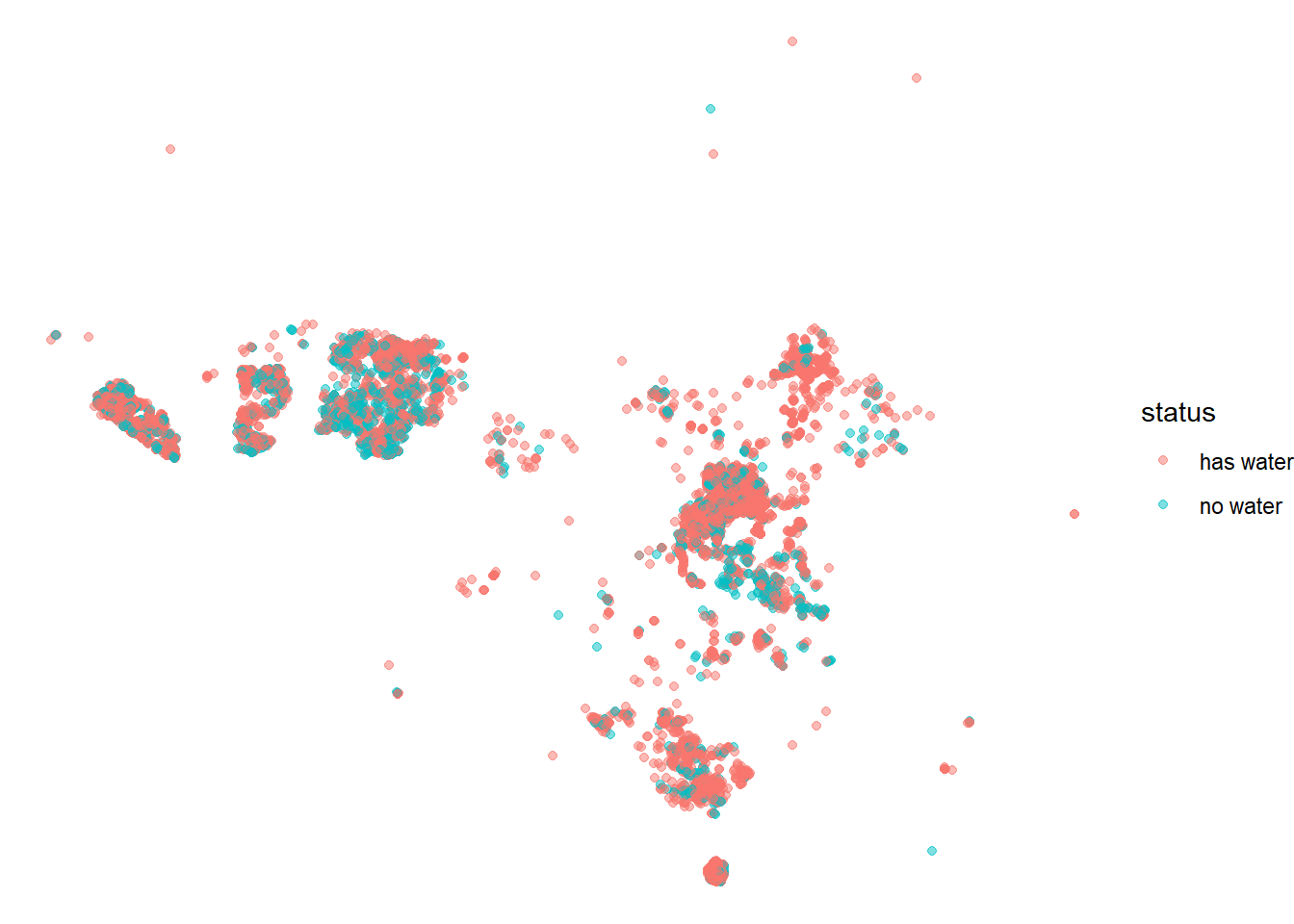
Here is the way for us to filter out the countries not in Africa:
africa_map <- map_data("world") %>%
  tibble() %>%
  mutate(continent = countrycode(region, origin = "country.name", destination = "continent")) %>%
  filter(continent == "Africa")

water %>%
  group_by(country) %>%
  summarize(across(lat:lon, mean)) %>%
  ungroup() %>%
  ggplot(aes(lon, lat)) +
  geom_polygon(data = africa_map, aes(long, lat, group = group), fill = "white", color = "grey") +
  geom_point() +
  geom_text(aes(label = country),
            hjust = -1,
            vjust = 0,
            check_overlap = T) +
  theme_map()
Since putting all the data points on the map is time consuming, here I just take some samples out by using sample_n() to give a sense of where the water sources are located.
water %>%
  sample_n(200000) %>%
  ggplot(aes(lon, lat)) +
  geom_polygon(data = africa_map, aes(long, lat, group = group), fill = "white", color = "grey") +
  geom_point(aes(color = status_id), alpha = 0.2, size = 0.1) +
  scale_color_discrete(guide = guide_legend(override.aes = list(size = 2, alpha = 1))) +
  theme_map() +
  labs(color = "status")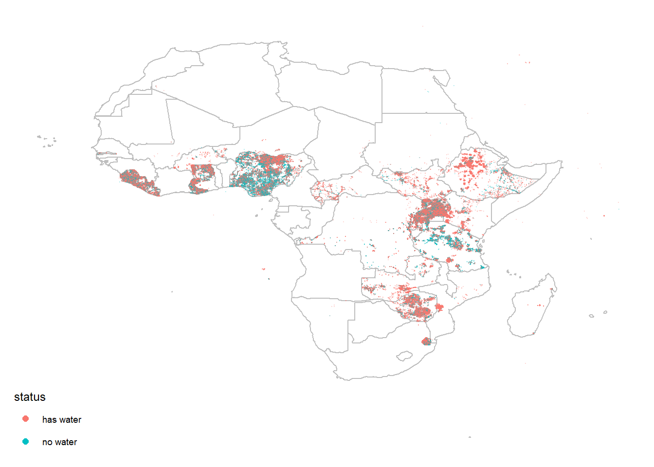
water %>%
  count(country, sort = T)
## # A tibble: 31 x 2
## country n
## <chr> <int>
## 1 Uganda 116589
## 2 Nigeria 83697
## 3 Sierra Leone 55840
## 4 Liberia 28657
## 5 Ethiopia 25031
## 6 Tanzania 24766
## 7 Swaziland 23913
## 8 Ghana 20969
## 9 Zimbabwe 17539
## 10 Kenya 11498
## # ... with 21 more rowsNigeria water sources:
water_nigeria <- water %>%
  filter(lon < 20,
         lat > 2) %>%
  filter(country == "Nigeria")

water_nigeria %>%
  ggplot(aes(lon, lat)) +
  geom_point(alpha = 0.1, size = 0.01) +
  borders(regions = "Nigeria") +
  theme_map() +
  ggtitle("Nigeria Water Sources")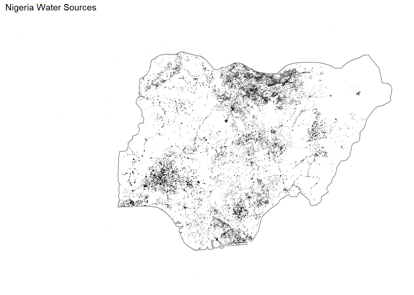
bounding_box <- c(left = 2, bottom = 4, right = 15, top = 13)
nigeria_map <- get_stamenmap(bounding_box, zoom = 8)

ggmap(nigeria_map) +
  geom_point(data = water_nigeria, aes(lon, lat, color = status_id), alpha = 0.1, size = 0.1) +
  borders(regions = "Nigeria") +
  theme_map() +
  labs(color = "status") +
  ggtitle("Nigeria Water Sources") +
  scale_color_discrete(guide = guide_legend(override.aes = list(size = 2, alpha = 1)))
water %>%
  filter(!is.na(water_source)) %>%
  count(water_source, status_id, sort = T) %>%
  mutate(water_source = fct_reorder(water_source, n, sum)) %>%
  ggplot(aes(n, water_source, fill = status_id)) +
  geom_col() +
  labs(x = "# of water sources",
       y = "",
       fill = "",
       title = "Water Sources and Their Counts")
water %>%
  filter(!is.na(install_year),
         fct_lump(country, n = 13) != "Other") %>%
  count(country, install_year, status_id, sort = T) %>%
  mutate(country = fct_reorder(country, -n, sum)) %>%
  ggplot(aes(install_year, n, fill = status_id)) +
  geom_area(alpha = 0.8) +
  facet_wrap(~ country) +
  theme(axis.text.x = element_text(angle = 90)) +
  labs(x = "install year",
       y = "# of water sources",
       fill = NULL,
       title = "# of water sources on install year and count")
water %>%
  filter(!is.na(installer)) %>%
  mutate(installer = str_remove(installer, " \\(UN\\)$")) %>%
  add_count(installer) %>%
  filter(n > 2000) %>%
  pairwise_cor(installer, country, sort = T) %>%
  ggplot(aes(item1, item2, fill = correlation)) +
  geom_tile() +
  theme(panel.grid = element_blank(),
        axis.text.x = element_text(angle = 90)) +
  scale_fill_gradient2(low = "red",
                       mid = "pink",
                       high = "green") +
  labs(x = NULL,
       y = NULL,
       title = "How installers are correlated within countries?")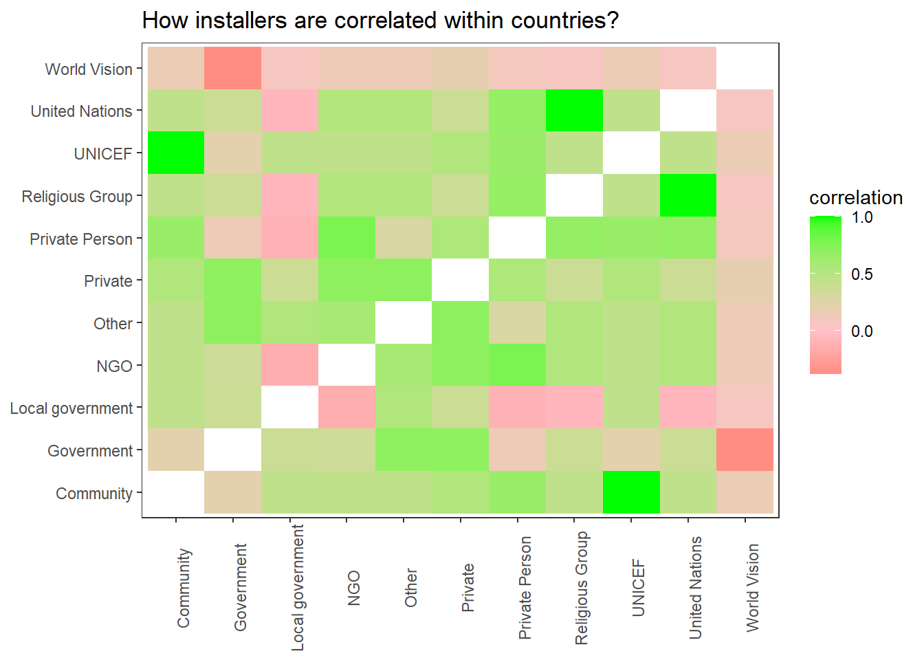
Here I am using tidymodels to train data, but there is something wrong with the recipe.
Split the data into training and testing:
set.seed(2022)

spl <- initial_split(water %>% filter(!is.na(install_year)), strata = status_id)
water_train <- training(spl)
water_test <- testing(spl)
Creating 10-fold CV:
set.seed(2022)
water_folds <- vfold_cv(water_train, strata = status_id)
Creating logistic regression and random forest algorithms:
log_spec <- logistic_reg() %>%
  set_engine("glm")

rand_spec <- rand_forest(trees = 1000) %>%
  set_mode("classification") %>%
  set_engine("ranger")
Setting up the recipe here:
water_rec <- recipe(status_id ~ facility_type + country + install_year,
                    data = water_train) %>%
  step_string2factor(status_id) %>%
  step_unknown(all_nominal_predictors()) %>%
  step_other(country, threshold = 0.1) %>%
  step_dummy(all_nominal_predictors())
Constructing the workflows:
water_wf <- workflow() %>%
  add_recipe(water_rec) %>%
  add_model(log_spec)

water_res <-  water_wf %>%
  fit_resamples(
    resamples = water_folds,
    control = control_resamples(save_pred = T)
  )

water_res %>%
  collect_metrics()
## # A tibble: 2 x 6
## .metric .estimator mean n std_err .config
## <chr> <chr> <dbl> <int> <dbl> <chr>
## 1 accuracy binary 0.773 10 0.000164 Preprocessor1_Model1
## 2 roc_auc binary 0.649 10 0.00121 Preprocessor1_Model1water_res %>%
collect_predictions() %>%
group_by(id) %>%
roc_curve(status_id, `.pred_has water`) %>%
autoplot()
Besides the logistic regression, random forest is used to train the data:
doParallel::registerDoParallel(cores = 8)

water_rand_wf <- workflow() %>%
  add_recipe(water_rec) %>%
  add_model(rand_spec)

water_rand_res <- water_rand_wf %>%
  fit_resamples(
    resamples = water_folds,
    control = control_resamples(save_pred = T)
  )

water_rand_res %>%
  collect_predictions() %>%
  group_by(id) %>%
  roc_curve(status_id, `.pred_has water`) %>%
autoplot() 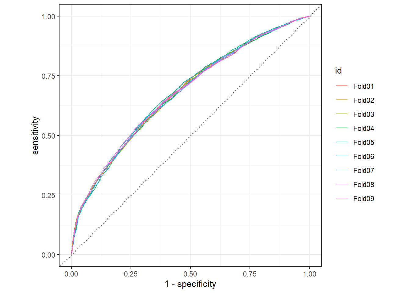
We can see that the random forest performs slightly better than the logistic regression.
final_fit <- water_rand_wf %>%
  last_fit(spl)

final_fit %>%
  collect_metrics()
## # A tibble: 2 x 4
## .metric .estimator .estimate .config
## <chr> <chr> <dbl> <chr>
## 1 accuracy binary 0.778 Preprocessor1_Model1
## 2 roc_auc binary 0.674 Preprocessor1_Model1