Comparing Linear Regression & Random Forest on NFL Data
In this blog post, I will use tidyverse and tidymodels to analyze some NFL data sets from TidyTuesday. I will use a simple linear regression and a slightly more complicated random forest model to make predictions, and through the predictive performance in both training and testing data, we can see that the linear regression model has high bias and the random forest model has the high variance.
library(tidyverse)
library(tidymodels)
theme_set(theme_bw())
attendance <- read_csv("https://raw.githubusercontent.com/rfordatascience/tidytuesday/master/data/2020/2020-02-04/attendance.csv")
standings <- read_csv("https://raw.githubusercontent.com/rfordatascience/tidytuesday/master/data/2020/2020-02-04/standings.csv")Join the two tibbles together:
nfl_joined <- attendance %>%
  left_join(
    standings,
    by = c("team", "team_name", "year")
  )

nfl_joined
## # A tibble: 10,846 x 20
## team team_name year total home away week weekly_attendan~ wins loss
## <chr> <chr> <dbl> <dbl> <dbl> <dbl> <dbl> <dbl> <dbl> <dbl>
## 1 Ariz~ Cardinals 2000 893926 387475 506451 1 77434 3 13
## 2 Ariz~ Cardinals 2000 893926 387475 506451 2 66009 3 13
## 3 Ariz~ Cardinals 2000 893926 387475 506451 3 NA 3 13
## 4 Ariz~ Cardinals 2000 893926 387475 506451 4 71801 3 13
## 5 Ariz~ Cardinals 2000 893926 387475 506451 5 66985 3 13
## 6 Ariz~ Cardinals 2000 893926 387475 506451 6 44296 3 13
## 7 Ariz~ Cardinals 2000 893926 387475 506451 7 38293 3 13
## 8 Ariz~ Cardinals 2000 893926 387475 506451 8 62981 3 13
## 9 Ariz~ Cardinals 2000 893926 387475 506451 9 35286 3 13
## 10 Ariz~ Cardinals 2000 893926 387475 506451 10 52244 3 13
## # ... with 10,836 more rows, and 10 more variables: points_for <dbl>,
## # points_against <dbl>, points_differential <dbl>, margin_of_victory <dbl>,
## # strength_of_schedule <dbl>, simple_rating <dbl>, offensive_ranking <dbl>,
## # defensive_ranking <dbl>, playoffs <chr>, sb_winner <chr>Weekly attendance per team:
nfl_joined %>%
  mutate(team = fct_reorder(team, weekly_attendance, na.rm = T)) %>%
  ggplot(aes(weekly_attendance, team, fill = team, color = team)) +
  geom_boxplot(alpha = 0.5) +
  theme(legend.position = "none",
        panel.grid = element_blank()) +
  labs(x = "weekly attendance",
       y = "",
       title = "Weekly Attendance Per Team")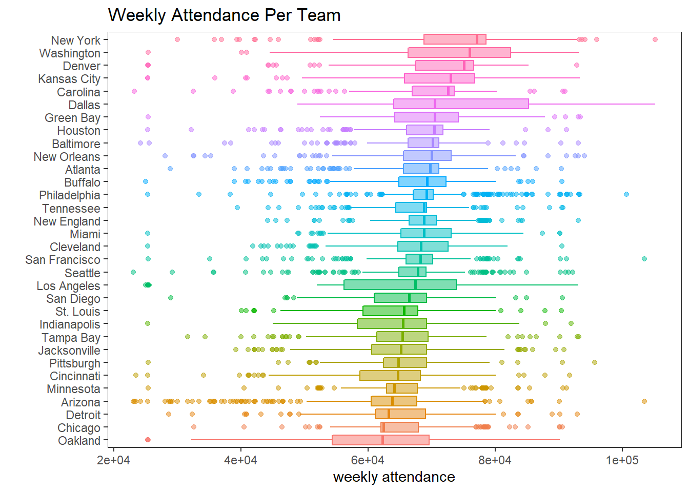
Weekly attendance per week:
nfl_joined %>%
  mutate(team = fct_reorder(team, weekly_attendance, na.rm = T)) %>%
  ggplot(aes(factor(week), weekly_attendance, fill = factor(week), color = factor(week))) +
  geom_boxplot(alpha = 0.5) +
  theme(legend.position = "none",
        panel.grid = element_blank()) +
  labs(x = "week",
       y = "weekly attendance",
       title = "Weekly Attendance Per Week")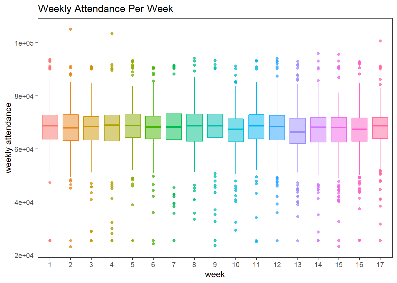
Data preparation
After following Julia Silge’s blog post link, the following data columns are used:
nfl_df <- nfl_joined %>%
  filter(!is.na(weekly_attendance)) %>%
  select(
    weekly_attendance, team_name, year, week,
    margin_of_victory, strength_of_schedule, playoffs
  )

nfl_df
## # A tibble: 10,208 x 7
## weekly_attendance team_name year week margin_of_victory strength_of_schedu~
## <dbl> <chr> <dbl> <dbl> <dbl> <dbl>
## 1 77434 Cardinals 2000 1 -14.6 -0.7
## 2 66009 Cardinals 2000 2 -14.6 -0.7
## 3 71801 Cardinals 2000 4 -14.6 -0.7
## 4 66985 Cardinals 2000 5 -14.6 -0.7
## 5 44296 Cardinals 2000 6 -14.6 -0.7
## 6 38293 Cardinals 2000 7 -14.6 -0.7
## 7 62981 Cardinals 2000 8 -14.6 -0.7
## 8 35286 Cardinals 2000 9 -14.6 -0.7
## 9 52244 Cardinals 2000 10 -14.6 -0.7
## 10 64223 Cardinals 2000 11 -14.6 -0.7
## # ... with 10,198 more rows, and 1 more variable: playoffs <chr>Data split:
set.seed(2022)

nfl_spl <- nfl_df %>%
  initial_split()

nfl_train <- training(nfl_spl)
nfl_test <- testing(nfl_spl)
Making the recipe:
nfl_rec <- recipe(weekly_attendance ~ ., data = nfl_train) Making the linear model:
lin_spec <- linear_reg() %>%
  set_engine("lm") %>%
  set_mode("regression")
Setting up the workflow:
lin_wf <- workflow() %>%
  add_recipe(nfl_rec) %>%
  add_model(lin_spec)
Fit the training data:
lin_fit <- lin_wf %>%
  fit(nfl_train)
After fitting the linear model, let’s use the random forest to fit the data.
Making the random forest model:
rand_spec <- rand_forest() %>%
  set_engine("ranger") %>%
  set_mode("regression")
Creating the random forest workflow:
rand_wf <- workflow() %>%
  add_recipe(nfl_rec) %>%
  add_model(rand_spec)
Train the random forest model:
rand_fit <- rand_wf %>%
  fit(nfl_train)
Comparing both models on the training data:
augment(rand_fit, nfl_train) %>%
  rmse(weekly_attendance, .pred) %>%
  mutate(model = "random forest") %>%
  bind_rows(
    augment(lin_fit, nfl_train) %>%
      rmse(weekly_attendance, .pred) %>%
      mutate(model = "linear regression")
  )
## # A tibble: 2 x 4
## .metric .estimator .estimate model
## <chr> <chr> <dbl> <chr>
## 1 rmse standard 6048. random forest
## 2 rmse standard 8199. linear regressionBased on the training data, the random forest performs much better than the linear regression model, and the metric used here is RMSE.
Comparing both models on the testing data:
augment(rand_fit, nfl_test) %>%
  rmse(weekly_attendance, .pred) %>%
  mutate(model = "random forest") %>%
  bind_rows(
    augment(lin_fit, nfl_test) %>%
      rmse(weekly_attendance, .pred) %>%
      mutate(model = "linear regression")
  )
## # A tibble: 2 x 4
## .metric .estimator .estimate model
## <chr> <chr> <dbl> <chr>
## 1 rmse standard 8728. random forest
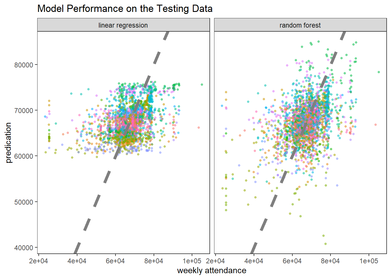
## 2 rmse standard 8671. linear regressionWhen evaluating the models on the testing data, however, linear regression performs better. This indicates that the random forest model has high variance.
Plotting the model predictions on the testing data:
augment(rand_fit, nfl_test) %>%
  mutate(model = "random forest") %>%
  bind_rows(
    augment(lin_fit, nfl_test) %>%
      mutate(model = "linear regression")
  ) %>%
  ggplot(aes(weekly_attendance, .pred, color = team_name)) +
  geom_point(size = 1, alpha = 0.5, show.legend = F) +
  geom_abline(lty = 2, size = 2, color = "grey50") +
  theme(panel.grid = element_blank()) +
  facet_wrap(~model) +
  labs(x = "weekly attendance",
       y = "predication",
       title = "Model Performance on the Testing Data")