K-Nearest Neighbors & Decision Tree on Hotel Bookings
In this blog post, I will analyze a hotel booking dataset from TidyTuesday, and some of the ideas presented are inspired by Julia Silge’s blog post (link) for learning purposes solely.
library(tidyverse)
library(tidymodels)
library(lubridate)
library(themis)
theme_set(theme_bw())
hotels <- read_csv("https://raw.githubusercontent.com/rfordatascience/tidytuesday/master/data/2020/2020-02-11/hotels.csv") %>%
inner_join(tibble(month = month.name,
month_abb = month.abb,
month_num = 1:12),
by = c("arrival_date_month" = "month")) %>%
mutate(month_abb = fct_reorder(month_abb, month_num))
hotels## # A tibble: 119,390 x 34
## hotel is_canceled lead_time arrival_date_year arrival_date_month
## <chr> <dbl> <dbl> <dbl> <chr>
## 1 Resort Hotel 0 342 2015 July
## 2 Resort Hotel 0 737 2015 July
## 3 Resort Hotel 0 7 2015 July
## 4 Resort Hotel 0 13 2015 July
## 5 Resort Hotel 0 14 2015 July
## 6 Resort Hotel 0 14 2015 July
## 7 Resort Hotel 0 0 2015 July
## 8 Resort Hotel 0 9 2015 July
## 9 Resort Hotel 1 85 2015 July
## 10 Resort Hotel 1 75 2015 July
## # ... with 119,380 more rows, and 29 more variables:
## # arrival_date_week_number <dbl>, arrival_date_day_of_month <dbl>,
## # stays_in_weekend_nights <dbl>, stays_in_week_nights <dbl>, adults <dbl>,
## # children <dbl>, babies <dbl>, meal <chr>, country <chr>,
## # market_segment <chr>, distribution_channel <chr>, is_repeated_guest <dbl>,
## # previous_cancellations <dbl>, previous_bookings_not_canceled <dbl>,
## # reserved_room_type <chr>, assigned_room_type <chr>, ...Booking status:
hotels %>%
  filter(reservation_status != "No-Show") %>%
  mutate(date = floor_date(reservation_status_date, unit = "month")) %>%
  count(date, reservation_status) %>%
  ggplot(aes(date, n, color = reservation_status)) +
  geom_line() +
  geom_point() +
  labs(x = NULL,
       y = "# of bookings",
       color = "reservation status",
       title = "# of Monthly Hotel Bookings")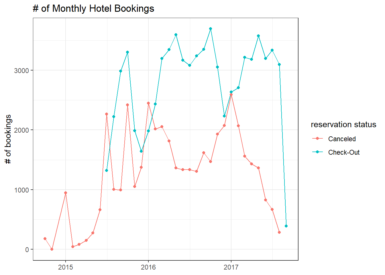
Monthly booking:
hotels %>%
  count(hotel, month_abb) %>%
  ggplot(aes(month_abb, n, fill = month_abb)) +
  geom_col(show.legend = F) +
  facet_wrap(~hotel, ncol = 1) +
  labs(x = "",
       y = "# of bookings",
       title = "# of Bookings per Month")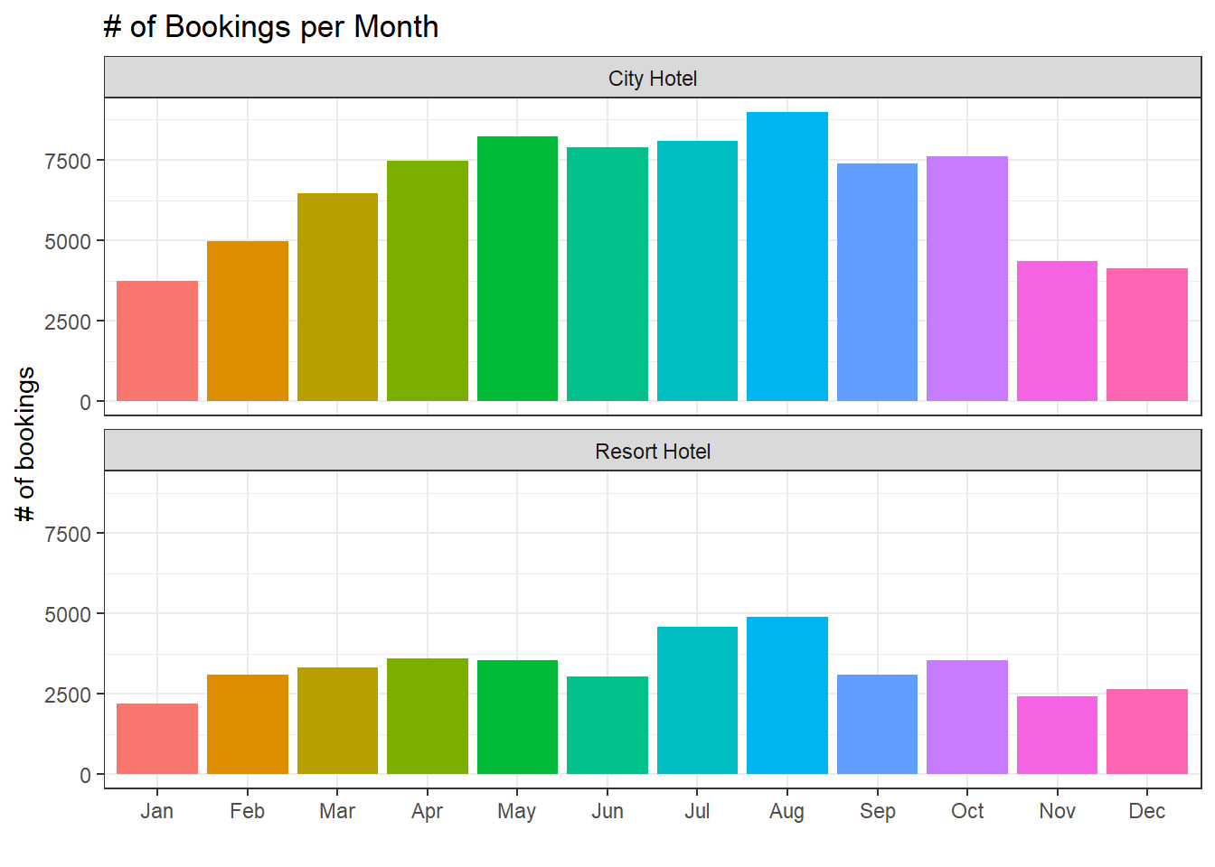
hotels %>%
  ggplot(aes(children)) +
  geom_histogram()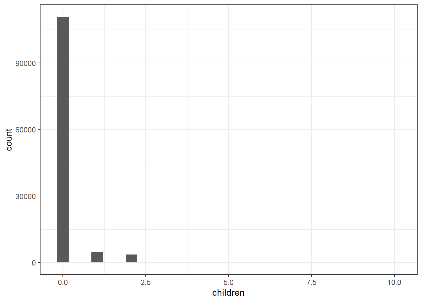
Since there are many reservations without having children, children can be encoded as a binary column specifying with or without children.
hotels_df <- hotels %>%
  mutate(children = factor(if_else(children > 0, "children", "none"))) %>%
  filter(!is.na(children))
Monthly booking with or without children:
hotels_df %>%
  count(hotel, month_abb, children) %>%
  group_by(hotel, children) %>%
  mutate(total_bookings = sum(n),
         pct_month = n/total_bookings) %>%
  ggplot(aes(month_abb, pct_month, fill = children)) +
  geom_col(position = "dodge") +
  scale_y_continuous(labels = scales::percent) +
  facet_wrap(~hotel, ncol = 1) +
  labs(x = "",
       y = "pct of bookings",
       fill = "",
title = "Percentage of Monthly Bookings") 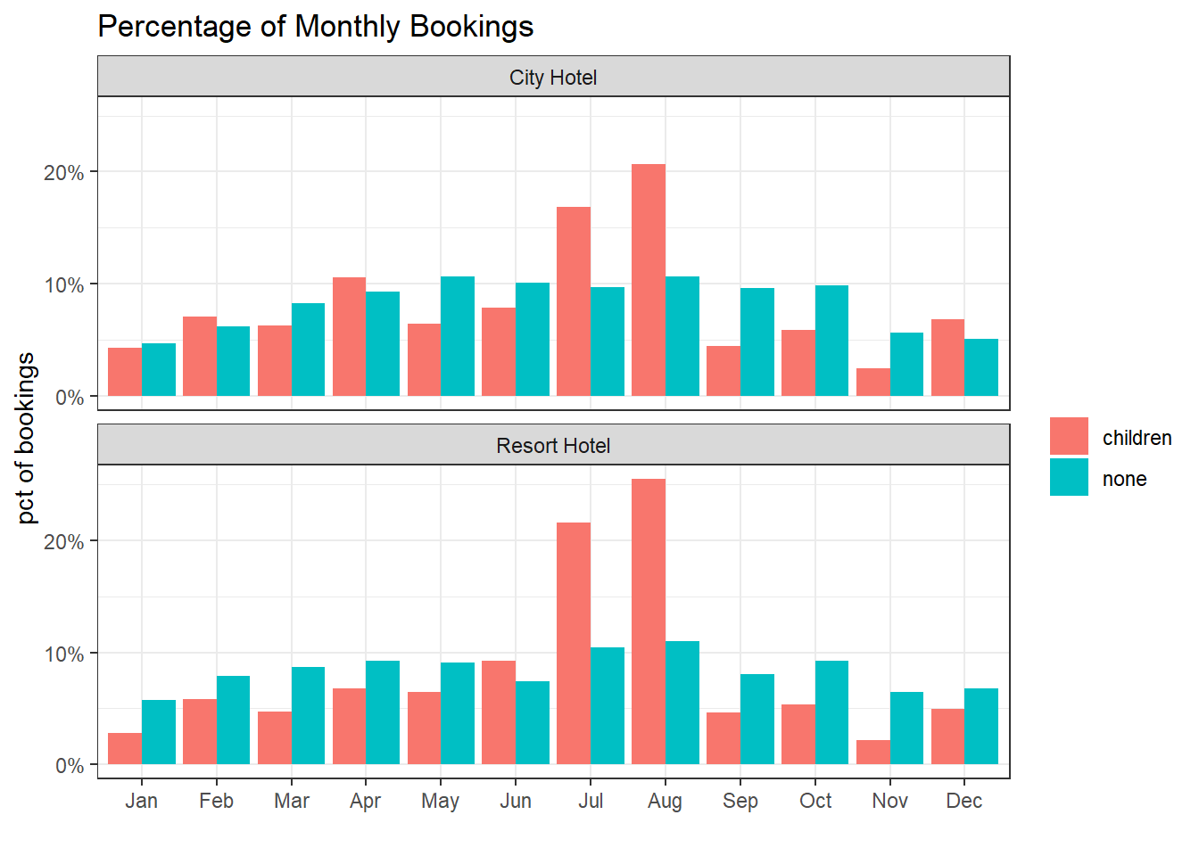
Clearly, July and August are the two popular months for bookings with children because of the summer.
Now we use some machine learning algorithms to classify if a booking has children or not.
hotels_df <- hotels_df %>%
  select(
    children, hotel, arrival_date_month, meal, adr, adults,
    required_car_parking_spaces, total_of_special_requests,
    stays_in_week_nights, stays_in_weekend_nights
  ) %>%
  mutate(across(where(is.character), factor))

hotels_df
## # A tibble: 119,386 x 10
## children hotel arrival_date_month meal adr adults required_car_par~
## <fct> <fct> <fct> <fct> <dbl> <dbl> <dbl>
## 1 none Resort Hotel July BB 0 2 0
## 2 none Resort Hotel July BB 0 2 0
## 3 none Resort Hotel July BB 75 1 0
## 4 none Resort Hotel July BB 75 1 0
## 5 none Resort Hotel July BB 98 2 0
## 6 none Resort Hotel July BB 98 2 0
## 7 none Resort Hotel July BB 107 2 0
## 8 none Resort Hotel July FB 103 2 0
## 9 none Resort Hotel July BB 82 2 0
## 10 none Resort Hotel July HB 106. 2 0
## # ... with 119,376 more rows, and 3 more variables:
## # total_of_special_requests <dbl>, stays_in_week_nights <dbl>,
## # stays_in_weekend_nights <dbl>- Split the data:
set.seed(2022)
doParallel::registerDoParallel()

hotels_spl <- hotels_df %>%
  initial_split(strata = "children")

hotels_train <- training(hotels_spl)
hotels_test <- testing(hotels_spl)


hotels_10fold <- vfold_cv(hotels_train, strata = "children", v = 10)- Make the recipe:
hotels_rec <- recipe(children ~ ., data = hotels_train) %>%
  step_dummy(all_nominal_predictors()) %>%
  step_zv(all_predictors()) %>%
step_downsample(children) - Models:
K-nearest neighbors:
knn_spec <- nearest_neighbor(neighbors = tune()) %>%
  set_mode("classification") %>%
  set_engine("kknn")
Tune neighbors:
knn_tune <- workflow() %>%
  add_model(knn_spec) %>%
  add_recipe(hotels_rec) %>%
  tune_grid(
    hotels_10fold,
    grid = crossing(neighbors = 10:15)
  )

autoplot(knn_tune)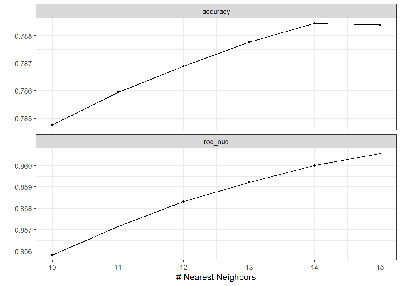
Finalize the workflow and use it to test the test data:
knn_final_fit <- workflow() %>%
  add_model(knn_spec) %>%
  add_recipe(hotels_rec) %>%
  finalize_workflow(select_best(knn_tune, "accuracy"))  %>%
  last_fit(hotels_spl)

knn_final_fit %>%
  unnest(.predictions) %>%
  roc_curve(children, .pred_children) %>%
  autoplot()
Decision tree model:
tree_spec <- decision_tree(tree_depth = tune(),
                           min_n = tune()) %>%
  set_mode("classification") %>%
  set_engine("rpart")
tree_tune <- workflow() %>%
add_model(tree_spec) %>%
add_recipe(hotels_rec) %>%
tune_grid(
hotels_10fold,
grid = crossing(tree_depth = c(10, 20, 30),
min_n = c(2, 10, 15, 20))
)
tree_res <- workflow() %>%
add_model(decision_tree() %>% set_mode("classification")) %>%
add_recipe(hotels_rec) %>%
fit_resamples(
hotels_10fold,
control = control_resamples(save_pred = T,
save_workflow = T)
)
tree_res %>%
unnest(.predictions) %>%
group_by(id) %>%
roc_curve(children, .pred_children) %>%
autoplot()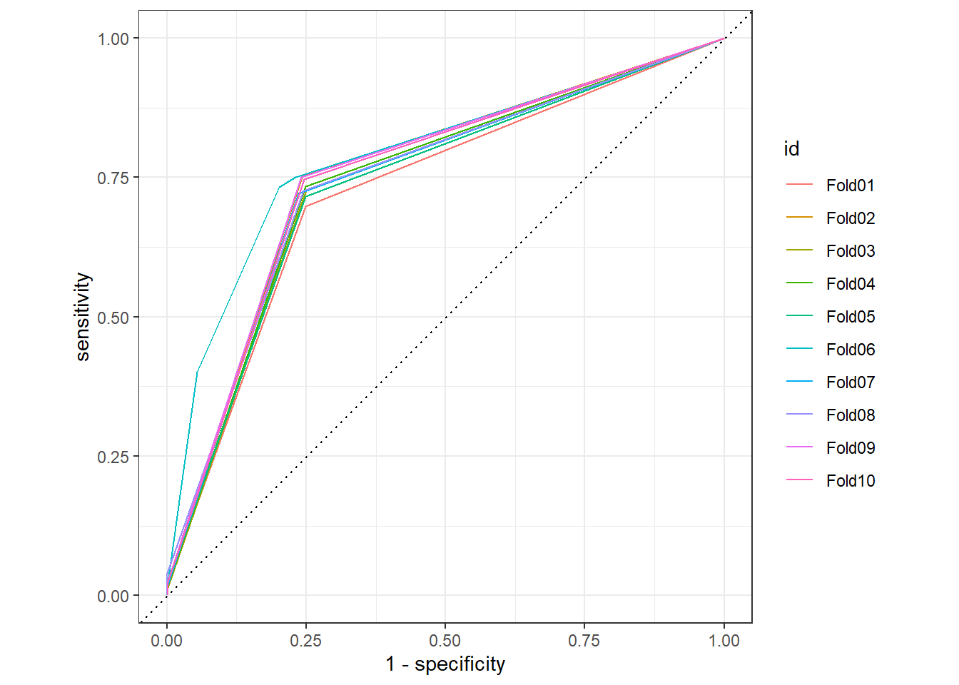
tree_test <- last_fit(workflow() %>%
                       add_model(decision_tree() %>% set_mode("classification")) %>%
                       add_recipe(hotels_rec),
hotels_spl)- Comparing models:
tree_test %>%
  unnest(.predictions) %>%
  mutate(model = "decision tree") %>%
  bind_rows(
    knn_final_fit %>%
      unnest(.predictions) %>%
      mutate(model = "knn")
  ) %>%
  group_by(model) %>%
  roc_curve(children, .pred_children) %>%
  ungroup() %>%
  mutate(model = fct_reorder(model, -sensitivity, sum)) %>%
  ggplot(aes(1 - specificity, sensitivity, color = model)) +
  geom_path(size = 1.5) +
  geom_abline(lty = 2, color = "grey50", size = 1.2) +
  ggtitle("ROC Curves for Decision Tree and KNN")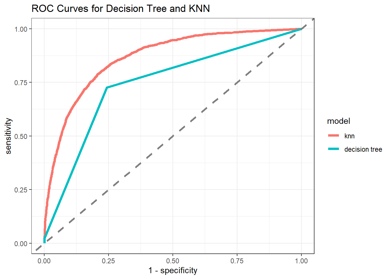
KNN is a better model for testing data than the decision tree.