Random Forest and XGboost on Predicting Continent
In this blog post, I will use a food consumption data set provided by TidyTuesday joined by a continent data set provided by the worlddatajoin package. You can download the package by typing devtools::install_github("PursuitOfDataScience/worlddatajoin") on the RStudio console. This is one of the blog posts I use the tidymodels meta-package to practice machine learning, and some of the ideas presented in this post are inspired by Julia Silge’s blog post (link).
library(tidyverse)
library(tidymodels)
library(worlddatajoin)
library(themis)
theme_set(theme_bw())
food_consumption <- read_csv("https://raw.githubusercontent.com/rfordatascience/tidytuesday/master/data/2020/2020-02-18/food_consumption.csv")
food_consumption## # A tibble: 1,430 x 4
## country food_category consumption co2_emmission
## <chr> <chr> <dbl> <dbl>
## 1 Argentina Pork 10.5 37.2
## 2 Argentina Poultry 38.7 41.5
## 3 Argentina Beef 55.5 1712
## 4 Argentina Lamb & Goat 1.56 54.6
## 5 Argentina Fish 4.36 6.96
## 6 Argentina Eggs 11.4 10.5
## 7 Argentina Milk - inc. cheese 195. 278.
## 8 Argentina Wheat and Wheat Products 103. 19.7
## 9 Argentina Rice 8.77 11.2
## 10 Argentina Soybeans 0 0
## # ... with 1,420 more rowsConsumption VS CO2 emission per country:
food_consumption %>%
  ggplot(aes(consumption, co2_emmission, color = food_category)) +
  geom_point() +
  geom_text(aes(label = country),
            hjust = 0,
            vjust = 1,
            check_overlap = T) +
  labs(x = "consumption (kg/person/year)",
       y = "CO2 Emission",
       color = "",
       title = "Food Consumption and CO2 Emission")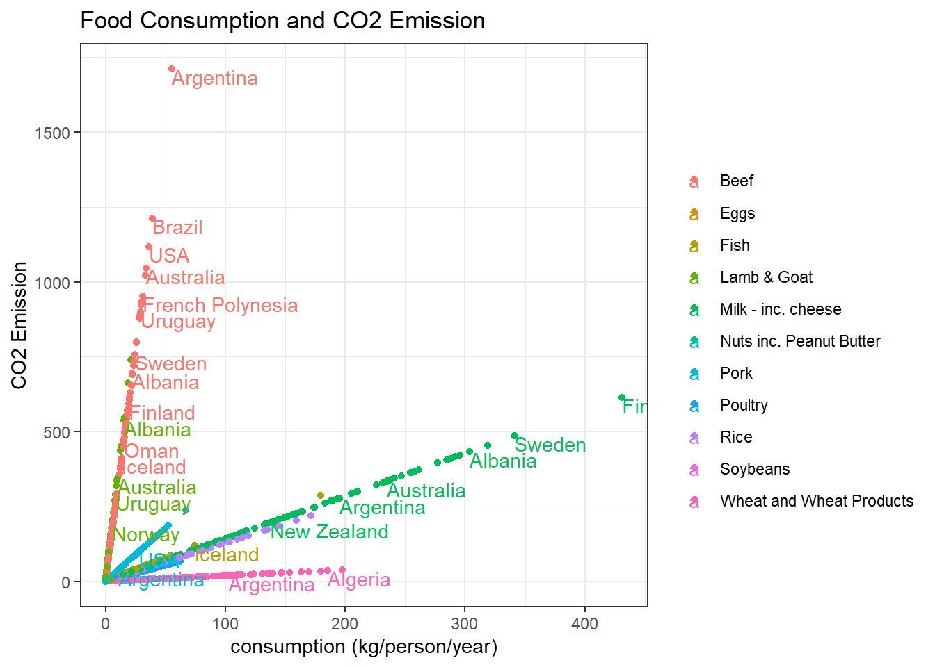
world_2020 <- worlddatajoin::world_data(2020) %>%
  distinct(country, continent)

food <- food_consumption %>%
  inner_join(world_2020, by = "country") %>%
  mutate(food_category = str_remove_all(food_category, "\\s+\\-inc.+$|\\sinc.+$"),
         food_category = str_remove(food_category, " -"))
Continent-wise CO2 emission and consumption:
food %>%
  pivot_longer(3:4) %>%
  mutate(name = str_replace(name, "_", " "),
         food_category = fct_reorder(food_category, value, sum)) %>%
  filter(value < 1000) %>%
  ggplot(aes(value, food_category, fill = continent, color = continent)) +
  geom_boxplot() +
  facet_wrap(~name, scales = "free_x") +
  labs(y = NULL,
       fill = NULL,
color = NULL) 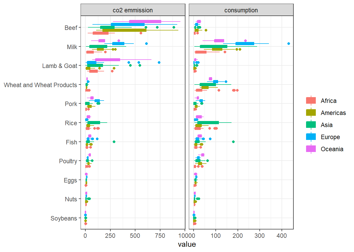
food_df <- food %>%
  select(-co2_emmission) %>%
  pivot_wider(names_from = food_category,
              values_from = consumption) %>%
  select(-country) %>%
  janitor::clean_names() %>%
  mutate(continent = if_else(continent == "Asia",
                             "Asia",
                             "Other"))

food_df
## # A tibble: 116 x 12
## continent pork poultry beef lamb_goat fish eggs milk wheat_and_wheat_pr~
## <chr> <dbl> <dbl> <dbl> <dbl> <dbl> <dbl> <dbl> <dbl>
## 1 Other 10.5 38.7 55.5 1.56 4.36 11.4 195. 103.
## 2 Other 24.1 46.1 33.9 9.87 17.7 8.51 234. 70.5
## 3 Other 10.9 13.2 22.5 15.3 3.85 12.4 304. 139.
## 4 Other 21.7 26.9 13.4 21.1 74.4 8.24 226. 72.9
## 5 Other 22.3 35.0 22.5 18.9 20.4 9.91 137. 76.9
## 6 Other 16.8 27.4 29.1 8.23 6.53 13.1 211. 109.
## 7 Other 43.6 21.4 29.9 1.67 23.1 14.6 255. 103.
## 8 Other 12.6 45 39.2 0.62 10.0 8.98 149. 53
## 9 Asia 10.4 18.4 23.4 9.56 5.21 8.29 288. 92.3
## 10 Other 37 16.6 24.6 1.41 23.9 13.4 341. 79.6
## # ... with 106 more rows, and 3 more variables: rice <dbl>, soybeans <dbl>,
## # nuts <dbl>Data Split:
set.seed(2022)
food_spl <- food_df %>%
  initial_split()

food_train <- training(food_spl)
food_test <- testing(food_spl)
Bootstrap:
food_boot <- bootstraps(food_df, times = 30)Make the recipe:
food_rec <- recipe(continent ~ ., data = food_train) %>%
  step_mutate(continent = factor(continent)) %>%
  step_downsample(continent)
Specify random forest model:
rand_spec <- rand_forest(
  trees = tune(),
  mtry = tune(),
  min_n = tune()
) %>%
  set_mode("classification") %>%
  set_engine("ranger")
Specify workflow:
rand_wf <- workflow() %>%
  add_recipe(food_rec) %>%
  add_model(rand_spec)
Tune the model:
rand_res <- rand_wf %>%
  tune_grid(
    resamples = food_boot,
    grid = crossing(
      trees = seq(500, 1500, 500),
      mtry = c(3,4,5,6,7),
      min_n = seq(3, 6)
    )
  )

autoplot(rand_res)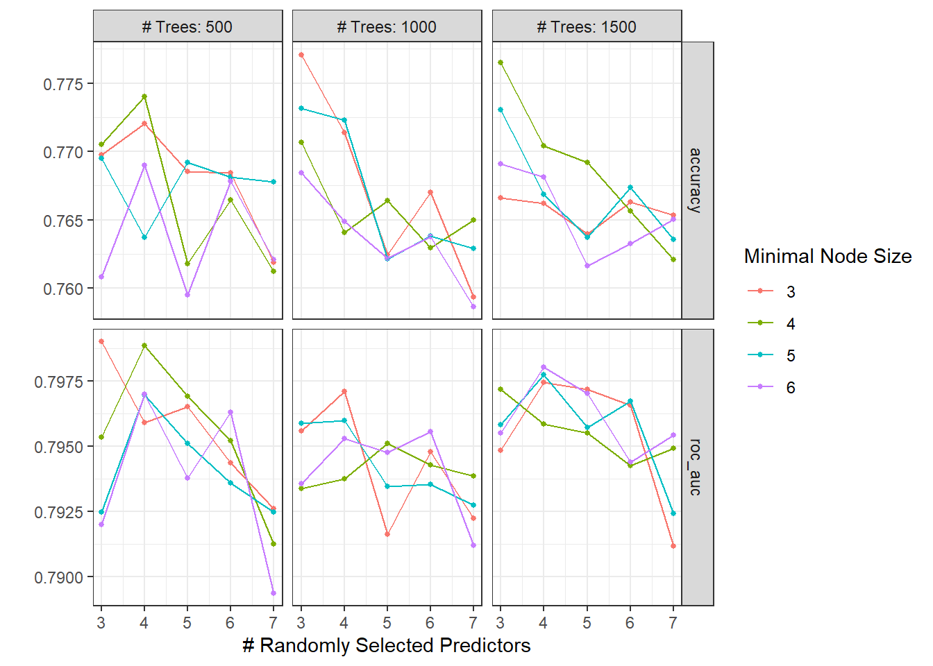
Fit the random forest model for the last time by training it on the training data and test it on the testing data:
rand_last_fit <- rand_wf %>%
  finalize_workflow(rand_res %>% select_best("accuracy")) %>%
  last_fit(food_spl)

rand_last_fit %>%
  collect_metrics()
## # A tibble: 2 x 4
## .metric .estimator .estimate .config
## <chr> <chr> <dbl> <chr>
## 1 accuracy binary 0.862 Preprocessor1_Model1
## 2 roc_auc binary 0.58 Preprocessor1_Model1The random forest does not perform well on the area under the ROC curve.
Using XGboost to walk through the same process as above:
xg_spec <- boost_tree(
  mtry = tune(),
  trees = tune(),
  tree_depth = tune(),
  learn_rate = 0.02
) %>%
  set_engine("xgboost") %>%
  set_mode("classification")

xg_wf <- workflow() %>%
  add_recipe(food_rec) %>%
  add_model(xg_spec)

xg_res <- xg_wf %>%
  tune_grid(
    food_boot,
    grid = crossing(
      trees = c(100, 300, 500),
      mtry = c(4,5,6),
      tree_depth = c(3, 6, 9)
    )
  )

autoplot(xg_res)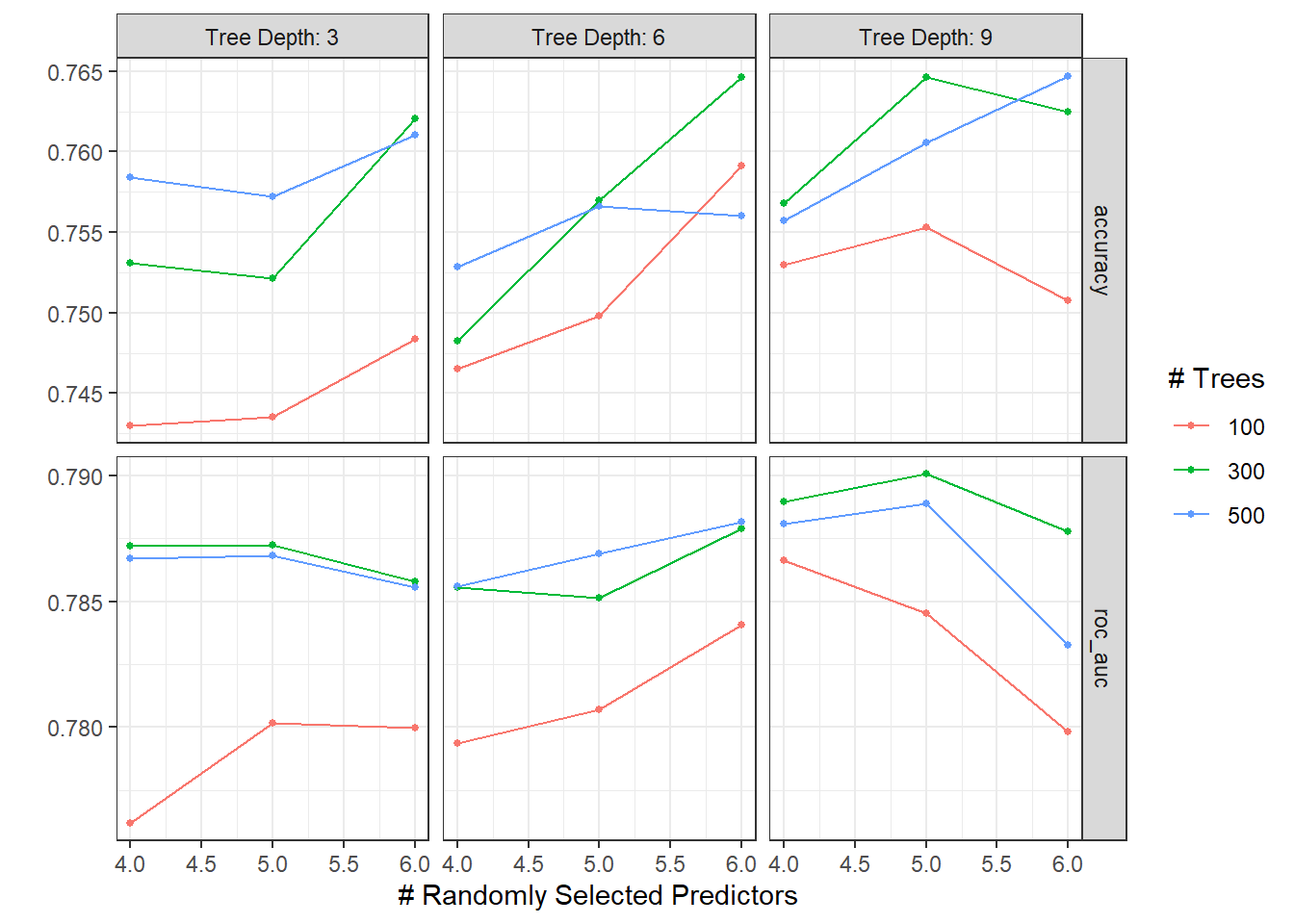
xg_wf %>%
  finalize_workflow(xg_res %>% select_best("roc_auc")) %>%
  last_fit(food_spl) %>%
  collect_metrics()
## # A tibble: 2 x 4
## .metric .estimator .estimate .config
## <chr> <chr> <dbl> <chr>
## 1 accuracy binary 0.862 Preprocessor1_Model1
## 2 roc_auc binary 0.59 Preprocessor1_Model1The XGboost roc_auc is slightly better than that of the random forest model.