Random Forest, LASSO, and XGboost on Classifying School Total Minority
This blog post will use three models, i.e., Random Forest, LASSO, and XGboost on data sets provided by TidyTuesday about college costs and minority information. Some ideas in this blog post are inspired by Julia Silge’s blog post (link).
library(tidyverse)
library(tidymodels)
library(geofacet)
library(scales)
theme_set(theme_bw())
tuition_cost <- readr::read_csv("https://raw.githubusercontent.com/rfordatascience/tidytuesday/master/data/2020/2020-03-10/tuition_cost.csv") %>%
rename(school = name) %>%
filter(type %in% c("Private", "Public"),
!is.na(state))
diversity_raw <- readr::read_csv("https://raw.githubusercontent.com/rfordatascience/tidytuesday/master/data/2020/2020-03-10/diversity_school.csv") %>%
rename(school = name) %>%
filter(!is.na(state))tuition_cost %>%
select(school, state, type, in_state_total, out_of_state_total) %>%
pivot_longer(cols = 4:5) %>%
mutate(name = str_replace_all(name, "_", " ")) %>%
ggplot(aes(value, type, fill = name)) +
geom_boxplot() +
facet_geo(~state) +
scale_x_continuous(n.breaks = 3,
labels = dollar) +
labs(x = NULL,
y = NULL,
fill = NULL,
title = "In/Out State Total Expenses per State")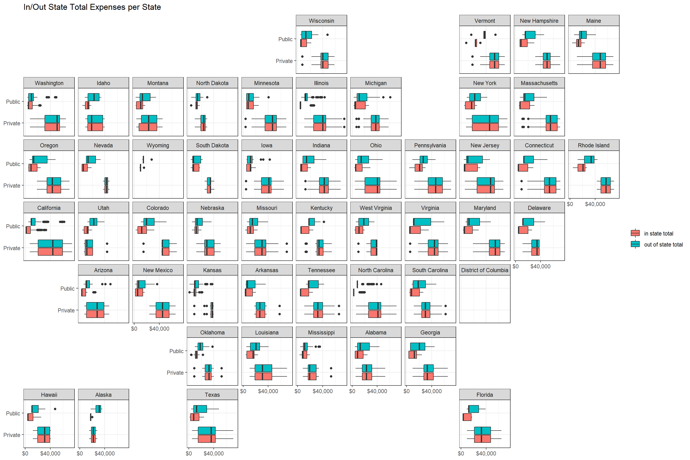
diversity_raw %>%
  mutate(category = fct_lump(category, n = 5, w = enrollment),
         pct_enrollment = enrollment / total_enrollment) %>%
  filter(category != "Other") %>%
  ggplot(aes(pct_enrollment, category, fill = category)) +
  geom_boxplot() +
  facet_geo(~state) +
  scale_x_continuous(labels = percent) +
  labs(x = "enrollment percentage",
       y = NULL,
       fill = NULL,
       title = "College Enrollment Category per State") +
  theme(axis.text.x = element_text(angle = 90))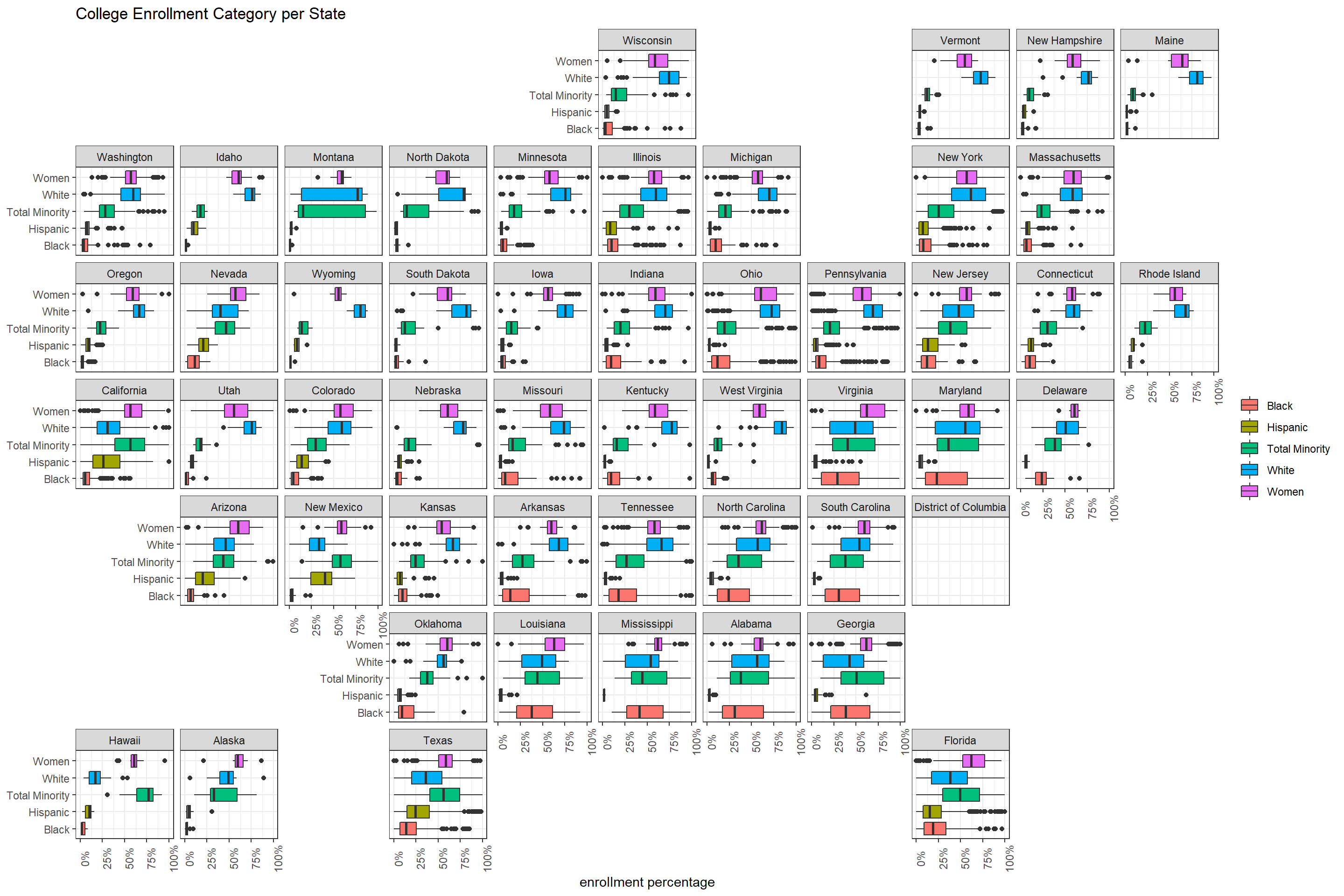
Here we categorize each school based on the percentage of Total Minority. If the percentage is above 30%, then total_minority is high. Otherwise, it is low.
university_df <- diversity_raw %>%
  filter(category == "Total Minority") %>%
  mutate(pct_minority = enrollment/total_enrollment,
         total_minority = if_else(pct_minority > 0.3, "high", "low")) %>%
  inner_join(tuition_cost,
            by = c("school", "state")) %>%
   select(-c(category, school, state, pct_minority, enrollment, contains("_total"))) %>%
  mutate(across(where(is.character), factor))

university_df
## # A tibble: 2,096 x 8
## total_enrollment total_minority state_code type degree_length room_and_board
## <dbl> <fct> <fct> <fct> <fct> <dbl>
## 1 81459 low VA Priv~ 4 Year 10478
## 2 66046 high FL Publ~ 2 Year NA
## 3 60767 high FL Publ~ 4 Year 9617
## 4 57821 low UT Priv~ 4 Year NA
## 5 51487 high VA Publ~ 2 Year NA
## 6 51313 high TX Publ~ 4 Year 10804
## 7 50320 high AZ Publ~ 4 Year 12648
## 8 50081 low MI Publ~ 4 Year 10322
## 9 49610 high FL Publ~ 4 Year 10882
## 10 49459 high FL Publ~ 4 Year 10120
## # ... with 2,086 more rows, and 2 more variables: in_state_tuition <dbl>,
## # out_of_state_tuition <dbl>Now let’s apply some machine learning algorithms to university_df to predict if a school is high or low on total_minority.
Split the data:
set.seed(2022)

university_spl <- university_df %>%
  initial_split()

university_train <- training(university_spl)
university_test <- testing(university_spl)

university_folds <- vfold_cv(university_train)
Make a recipe for the models:
university_rec <- recipe(total_minority ~ ., data = university_train) %>%
  step_impute_linear(room_and_board)
Random Forest and its workflow:
rand_spec <- rand_forest(trees = tune(),
            mtry = tune(),
            min_n = tune()) %>%
  set_mode("classification") %>%
  set_engine("ranger")

rand_wf <- workflow() %>%
  add_model(rand_spec) %>%
  add_recipe(university_rec)
Tune the random forest model:
rand_res <- rand_wf %>%
  tune_grid(
    university_folds,
    grid = crossing(
      trees = seq(500, 1500, 500),
      mtry = c(2, 3, 4, 5, 6),
      min_n = seq(3, 10, 2)
    )
  )

autoplot(rand_res)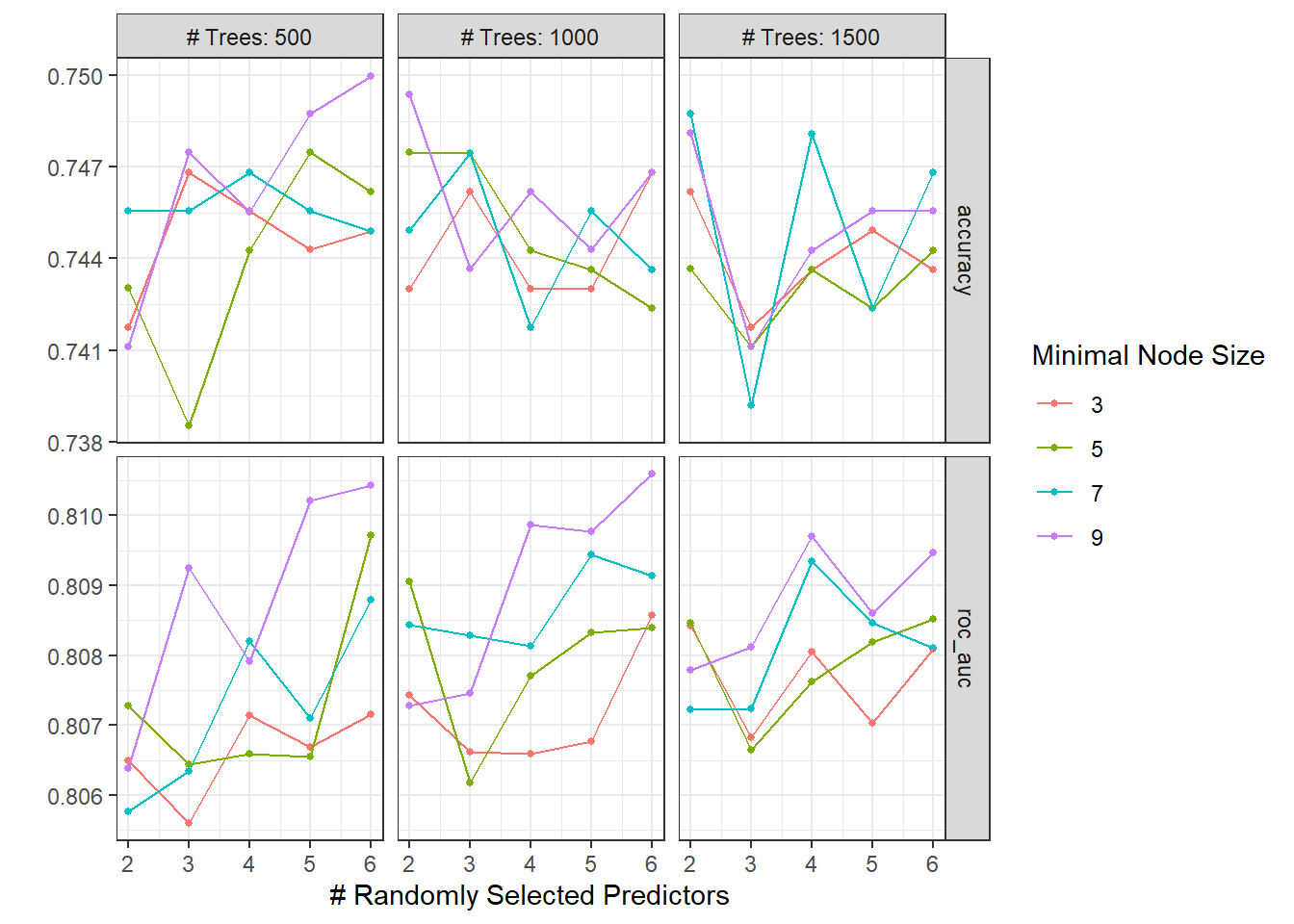
Final Fit and the ROC curve:
rand_last_fit <- rand_wf %>%
  finalize_workflow(rand_res %>% select_best("roc_auc")) %>%
  last_fit(university_spl)

rand_last_fit %>%
  collect_predictions() %>%
  roc_curve(total_minority, .pred_high) %>%
  autoplot()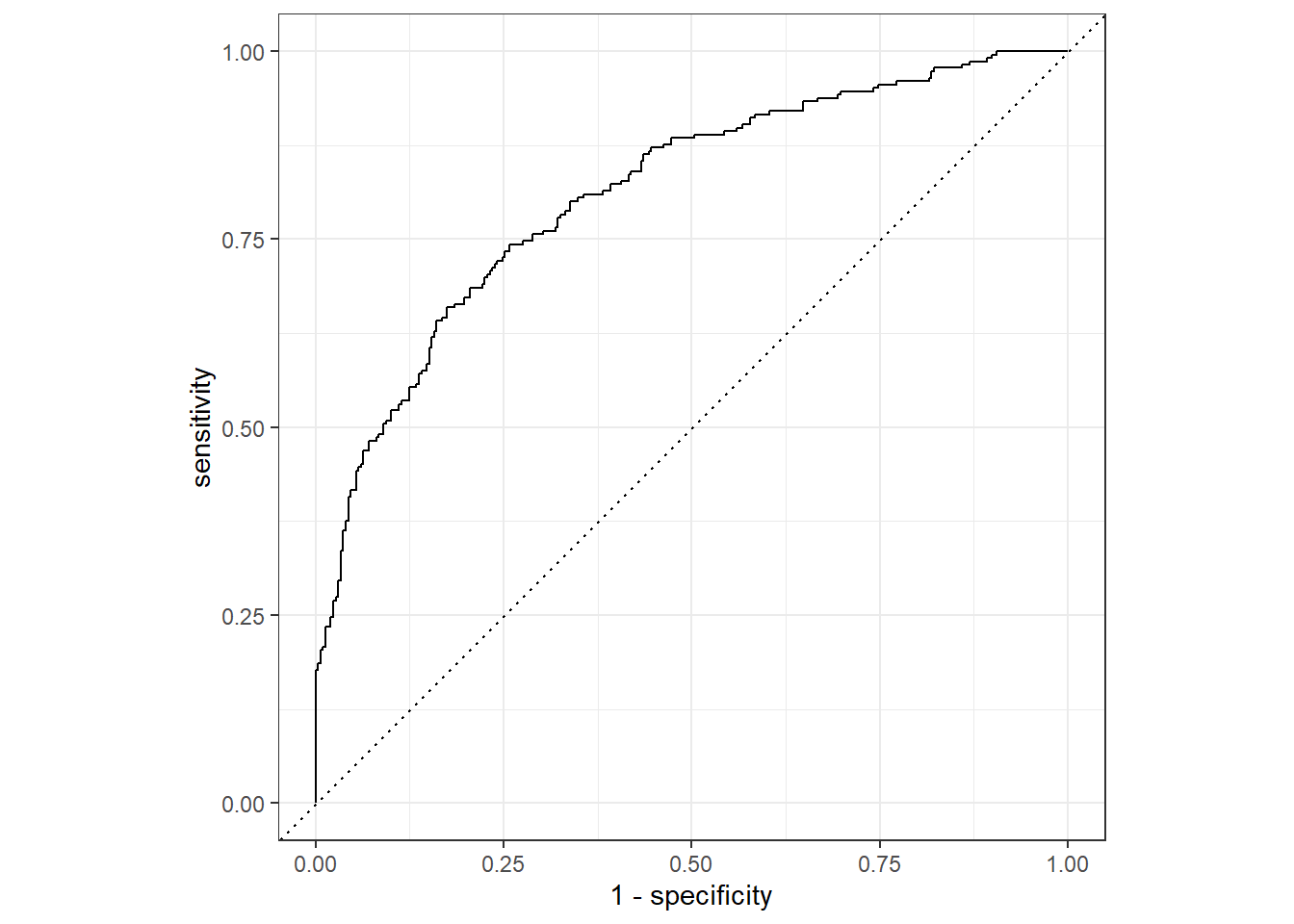
Lasso model:
log_spec <- logistic_reg(penalty = tune()) %>%
  set_engine("glmnet")

log_wf <- workflow() %>%
  add_model(log_spec) %>%
  add_recipe(university_rec %>%
               step_dummy(all_nominal_predictors()))

log_res <- log_wf %>%
  tune_grid(
    university_folds,
    grid = crossing(
      penalty = 10 ^ seq(-7, -0.5, 0.5)
    )
  )

autoplot(log_res)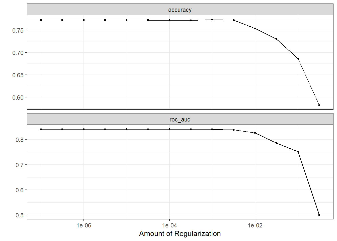
log_last_fit <- log_wf %>%
  finalize_workflow(log_res %>%
                      select_by_one_std_err(metric = "roc_auc", desc(penalty))
                    ) %>%
  last_fit(university_spl)

log_last_fit %>%
  collect_predictions() %>%
  roc_curve(total_minority, .pred_high) %>%
  autoplot()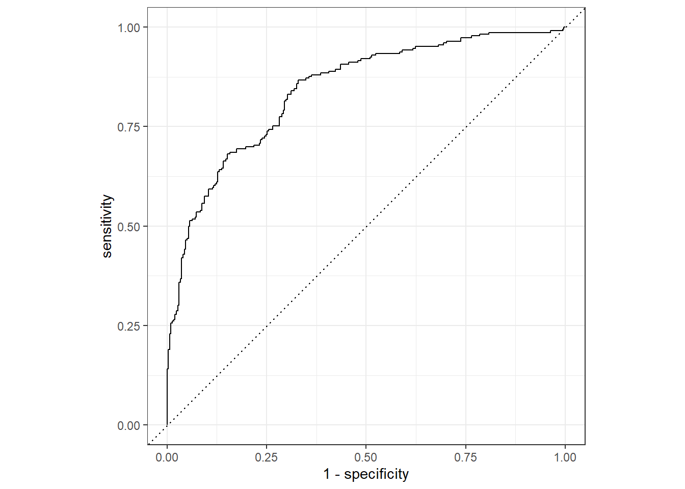
XGBoost:
xg_spec <- boost_tree(
  trees = tune(),
  min_n = tune(),
  mtry = tune(),
  learn_rate = 0.02
) %>%
  set_engine("xgboost") %>%
  set_mode("classification")

xg_wf <- workflow() %>%
  add_model(xg_spec) %>%
  add_recipe(university_rec %>%
               step_dummy(all_nominal_predictors()))

xg_res <- xg_wf %>%
  tune_grid(
    university_folds,
    grid = crossing(
      trees = seq(500, 1500, 500),
      mtry = c(2, 4, 6, 8, 10),
      min_n = c(3, 5, 7, 9)
    )
  )

autoplot(xg_res)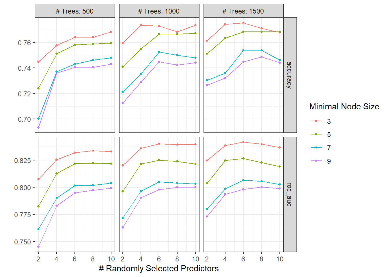
xg_last_fit <- xg_wf %>%
  finalize_workflow(xg_res %>%
                      select_best("roc_auc")) %>%
  last_fit(university_spl)

xg_last_fit %>%
  collect_predictions() %>%
  roc_curve(total_minority, .pred_high) %>%
  autoplot()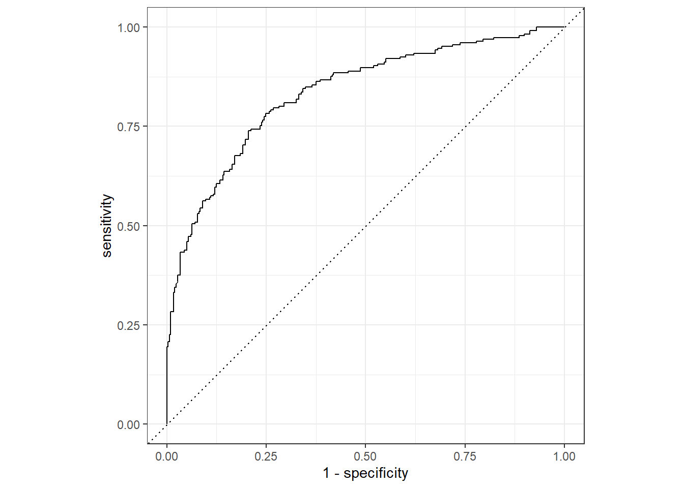
Comparing three models together:
select_predictions <- function(tbl){
  tbl %>%
    collect_predictions() %>%
    select(.pred_high, total_minority)
}

rand_last_fit %>%
  select_predictions() %>%
  mutate(mod = "Random Forest") %>%
  bind_rows(
    log_last_fit %>%
      select_predictions() %>%
      mutate(mod = "Logistic Regression")
  ) %>%
  bind_rows(
    xg_last_fit %>%
      select_predictions() %>%
      mutate(mod = "XGBoost")
  ) %>%
  group_by(mod) %>%
  roc_curve(total_minority, .pred_high) %>%
  ungroup() %>%
  ggplot(aes(1 - specificity, sensitivity, color = mod)) +
  geom_path(size = 2, alpha = 0.5) +
  geom_abline(lty = 2, color = "grey50", size = 2) +
  labs(color = "model",
       title = "ROC Curves for Three Tuned Models")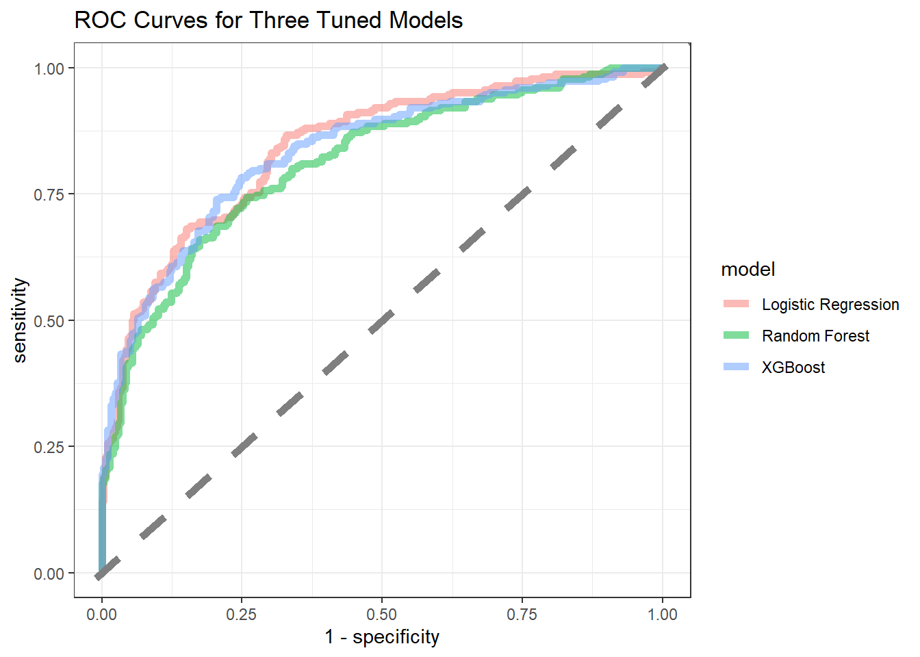
Three models perform very similarly on classifying whether a school is high or low on total minority, with XGboost slighly better.