Random Forest on Classifying San Francisco Trees

In this blog post, I will use random forest to classify a multi-classification problem on SF Trees provided by TidyTuesday. As always, tidyverse and tidymodels meta-packages will be used to process data and build machine learning model respectively.

library(tidyverse)
library(tidymodels)
theme_set(theme_bw())

sf_trees <- read_csv('https://raw.githubusercontent.com/rfordatascience/tidytuesday/master/data/2020/2020-01-28/sf_trees.csv') %>%
  mutate(species = str_remove(species, "\\s::.*"),
         site_info = str_remove(site_info, "\\s*:\\s*.*$"),
         legal_status = fct_lump(legal_status, n = 3)) %>%
  filter(longitude > -125,
         latitude > 37.7,
         !is.na(legal_status)) %>%
  select(-c(dbh, plot_size, address)) 

The tree locations:

sf_trees %>%
  ggplot(aes(longitude, latitude, color = legal_status)) +
  geom_point(alpha = 0.2, size = 0.5) +
  theme_void() +
  labs(color = "legal status",
       title = "Where the trees are located per legal status?")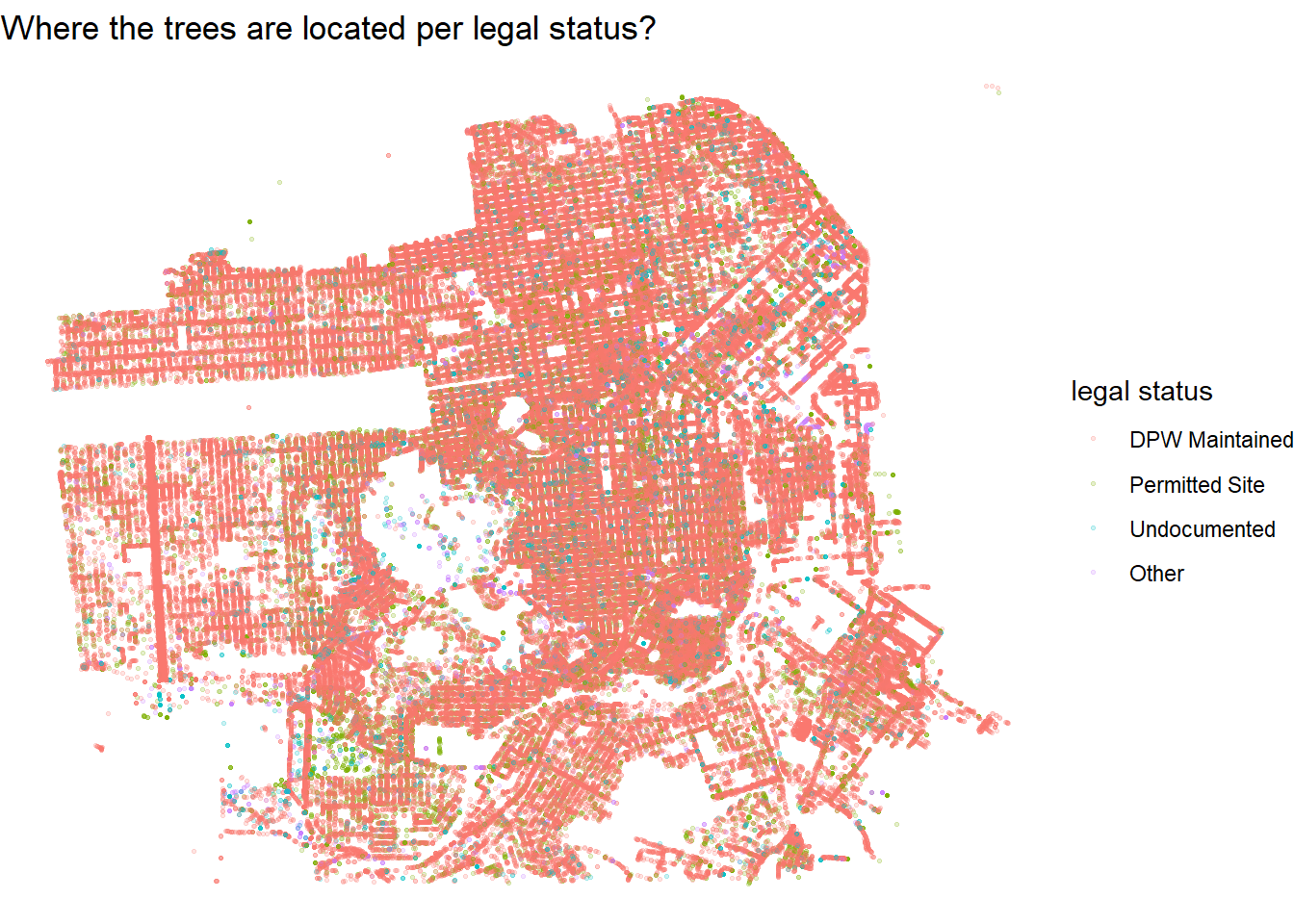 

I’d like to use random forest to predict the legal status of for trees.

Split the data:

set.seed(2022)

tree_spl <- sf_trees %>%
  initial_split(strata = "legal_status")

tree_train <- training(tree_spl)
tree_test <- testing(tree_spl)

tree_folds <- vfold_cv(tree_train, v = 3, strata = "legal_status")

Make the recipe:

tree_rec <- recipe(legal_status ~ ., data = tree_train) %>%
  add_role(tree_id, new_role = "id") %>%
  step_date(date, features = "year") %>%
  step_rm(date) %>%
  step_impute_mean(date_year, site_order) %>%
  step_novel(caretaker) %>%
  step_unknown(caretaker) %>%
  step_other(site_info, species, caretaker, threshold = 0.01) %>%
  step_dummy(all_nominal_predictors())

What I learned from making this recipe is that there are missing values for some columns in the testing data but not on the training data. step_novel() is a fantastic function to handle this tricky situation.

Specify the random forest model:

tree_spec <- rand_forest(
  trees = 500,
  mtry = tune(),
  min_n = tune()
) %>%
  set_mode("classification") %>%
  set_engine("ranger")

Specify the random forest workflow:

tree_wf <- workflow() %>%
  add_recipe(tree_rec) %>%
  add_model(tree_spec)

Tune the model:

doParallel::registerDoParallel(cores = 4)

tree_res <- tree_wf %>%
  tune_grid(
    tree_folds,
    grid = crossing(
      mtry = seq(2, 17, 2),
      min_n = c(2, 5)
    )
  )
  

autoplot(tree_res)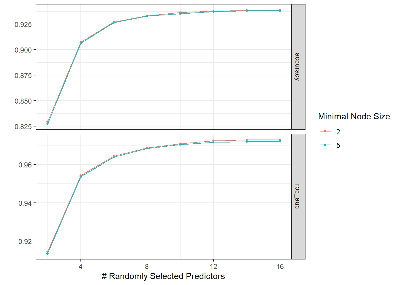

Due to the volume of the data, the code chunk above took a long time to finish.

Fit the model last time on the training data and test it on the testing data:

tree_last_fit <- tree_wf %>%
  finalize_workflow(tree_res %>%
                      select_best("roc_auc")) %>%
  last_fit(tree_spl)

tree_last_fit 

## # Resampling results
## # Manual resampling 
## # A tibble: 1 x 6
##   splits                 id            .metrics .notes   .predictions .workflow 
##   <list>                 <chr>         <list>   <list>   <list>       <list>    
## 1 <split [142477/47493]> train/test s~ <tibble> <tibble> <tibble>     <workflow>

Collect metrics:

tree_last_fit %>%
  collect_metrics()

## # A tibble: 2 x 4
##   .metric  .estimator .estimate .config             
##   <chr>    <chr>          <dbl> <chr>               
## 1 accuracy multiclass     0.947 Preprocessor1_Model1
## 2 roc_auc  hand_till      0.977 Preprocessor1_Model1

The model performs fantastically well.

The ROC curves:

tree_last_fit %>%
  collect_predictions() %>%
  roc_curve(legal_status, `.pred_DPW Maintained`:`.pred_Other`) %>% 
  autoplot()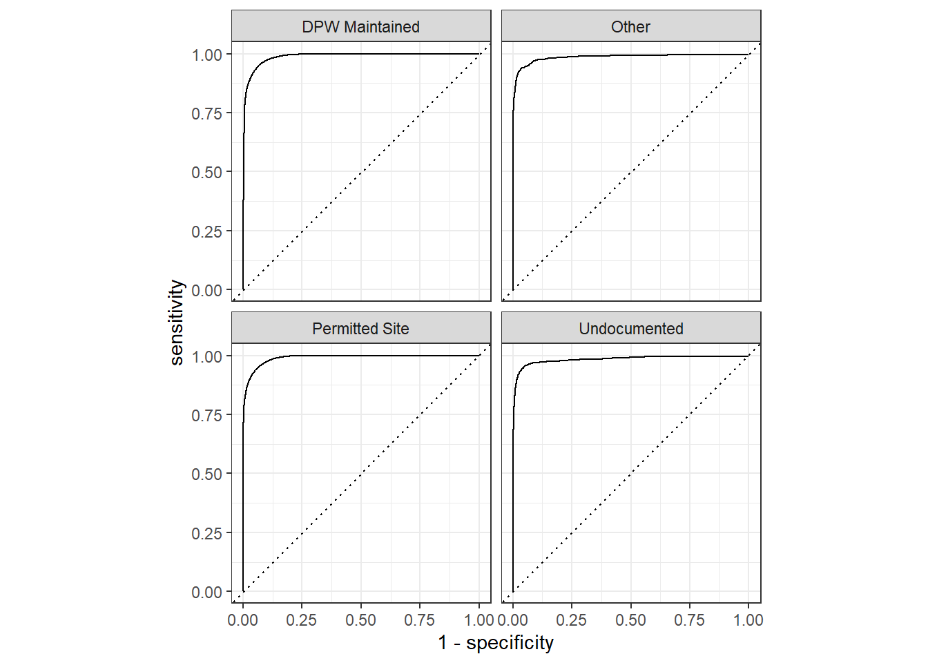

Since this is a multiple class problem, there are four ROC curves present above.

tree_last_fit %>%
  collect_predictions() %>%
  select(.pred_class, legal_status) %>%
  mutate(result = if_else(.pred_class == legal_status, "correct", "incorrect")) %>%
  bind_cols(tree_test) %>%
  ggplot(aes(longitude, latitude, color = result)) +
  geom_point(alpha = 0.5, size = 0.1) +
  theme_void() +
  scale_color_manual(values = c("gray80", "darkred")) +
  labs(color = "classification result")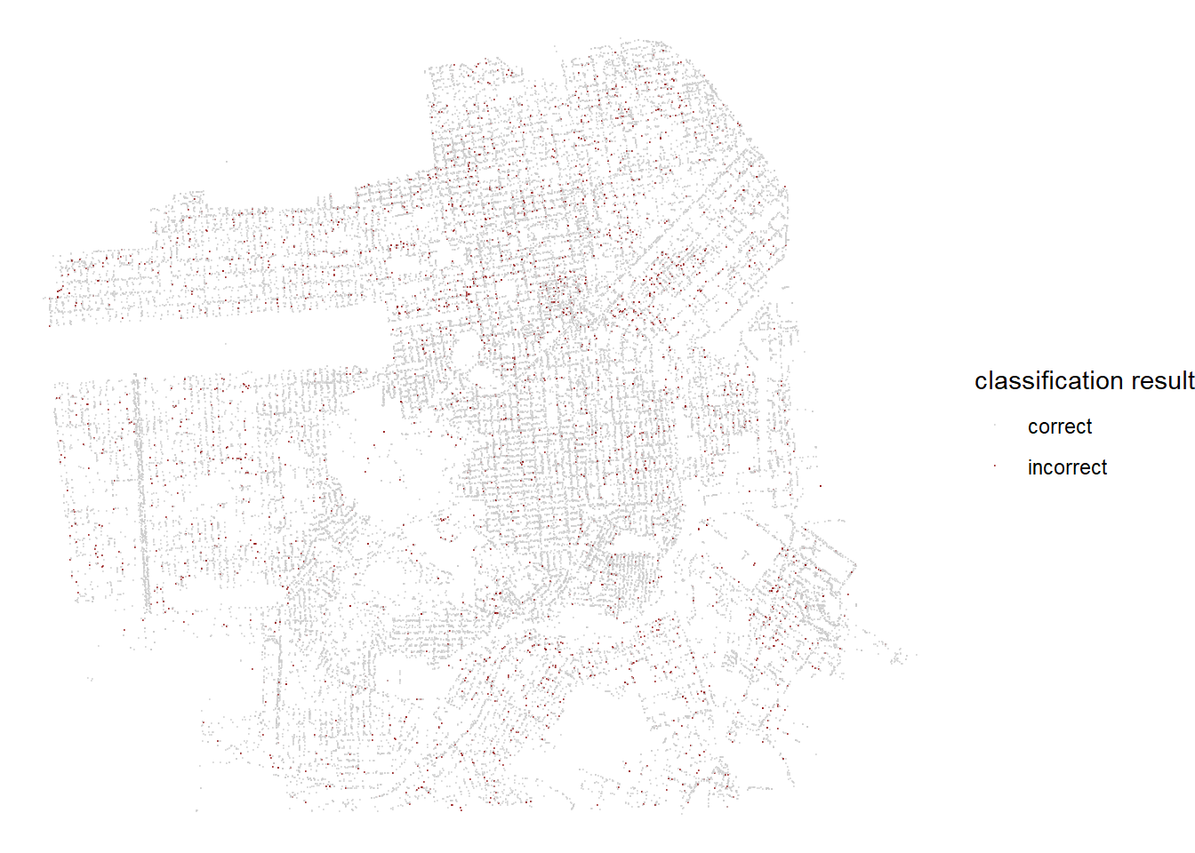

Combining all the predictions from the testing data and making a map on where the trees are classified correctly and incorrectly. This plot is inspired by Julia Silge’s blog post on analyzing the same data set. You can find her blog here.