Using LASSO to Predict Monthly Brew Materials
Mon, May 23, 2022
5-minute read
In this blog post, I will use a data set about beer brewing materials provided by TidyTuesday to make prediction for the monthly barrels of several beer materials. The tidymodels meta-package will be used, with bootstrap as the resampling technique.
library(tidyverse)
library(tidymodels)
library(lubridate)
theme_set(theme_bw())
brewing_materials_raw <- read_csv("https://raw.githubusercontent.com/rfordatascience/tidytuesday/master/data/2020/2020-03-31/brewing_materials.csv")
brewing_materials_raw## # A tibble: 1,440 x 9
## data_type material_type year month type month_current month_prior_year
## <chr> <chr> <dbl> <dbl> <chr> <dbl> <dbl>
## 1 Pounds of Mat~ Grain Produc~ 2008 1 Malt~ 374165152 365300134
## 2 Pounds of Mat~ Grain Produc~ 2008 1 Corn~ 57563519 41647092
## 3 Pounds of Mat~ Grain Produc~ 2008 1 Rice~ 72402143 81050102
## 4 Pounds of Mat~ Grain Produc~ 2008 1 Barl~ 3800844 2362162
## 5 Pounds of Mat~ Grain Produc~ 2008 1 Whea~ 1177186 1195381
## 6 Pounds of Mat~ Total Grain ~ 2008 1 Tota~ 509108844 491554871
## 7 Pounds of Mat~ Non-Grain Pr~ 2008 1 Suga~ 78358212 83664091
## 8 Pounds of Mat~ Non-Grain Pr~ 2008 1 Hops~ 4506546 2037754
## 9 Pounds of Mat~ Non-Grain Pr~ 2008 1 Hops~ 621912 411166
## 10 Pounds of Mat~ Non-Grain Pr~ 2008 1 Other 1291615 766735
## # ... with 1,430 more rows, and 2 more variables: ytd_current <dbl>,
## # ytd_prior_year <dbl>Clean and process brewing_materials_raw:
brewing_materials <- brewing_materials_raw %>%
  filter(type %in% c("Malt and malt products",
                     "Sugar and syrups",
                     "Rice and rice products",
                     "Barley and barley products",
                     "Wheat and wheat products")) %>%
  select(year, month, type, month_prior_year, month_current)

brewing_materials
## # A tibble: 600 x 5
## year month type month_prior_year month_current
## <dbl> <dbl> <chr> <dbl> <dbl>
## 1 2008 1 Malt and malt products 365300134 374165152
## 2 2008 1 Rice and rice products 81050102 72402143
## 3 2008 1 Barley and barley products 2362162 3800844
## 4 2008 1 Wheat and wheat products 1195381 1177186
## 5 2008 1 Sugar and syrups 83664091 78358212
## 6 2008 2 Malt and malt products 350035966 355687578
## 7 2008 2 Rice and rice products 75004651 66061597
## 8 2008 2 Barley and barley products 2573584 3236714
## 9 2008 2 Wheat and wheat products 1074183 1240983
## 10 2008 2 Sugar and syrups 86331629 80188744
## # ... with 590 more rowsEDA:
brewing_materials %>%
  mutate(year_month = ym(paste(year, month, sep = "-"))) %>%
  ggplot(aes(year_month, month_current, color = type)) +
  geom_line() +
  geom_point() +
  facet_wrap(~type, scales = "free_y", ncol = 1) +
  theme(legend.position = "none",
        panel.grid = element_blank()) +
  labs(x = NULL,
       y = "current number of monthly barrels",
       title = "Monthly Barrels per Type")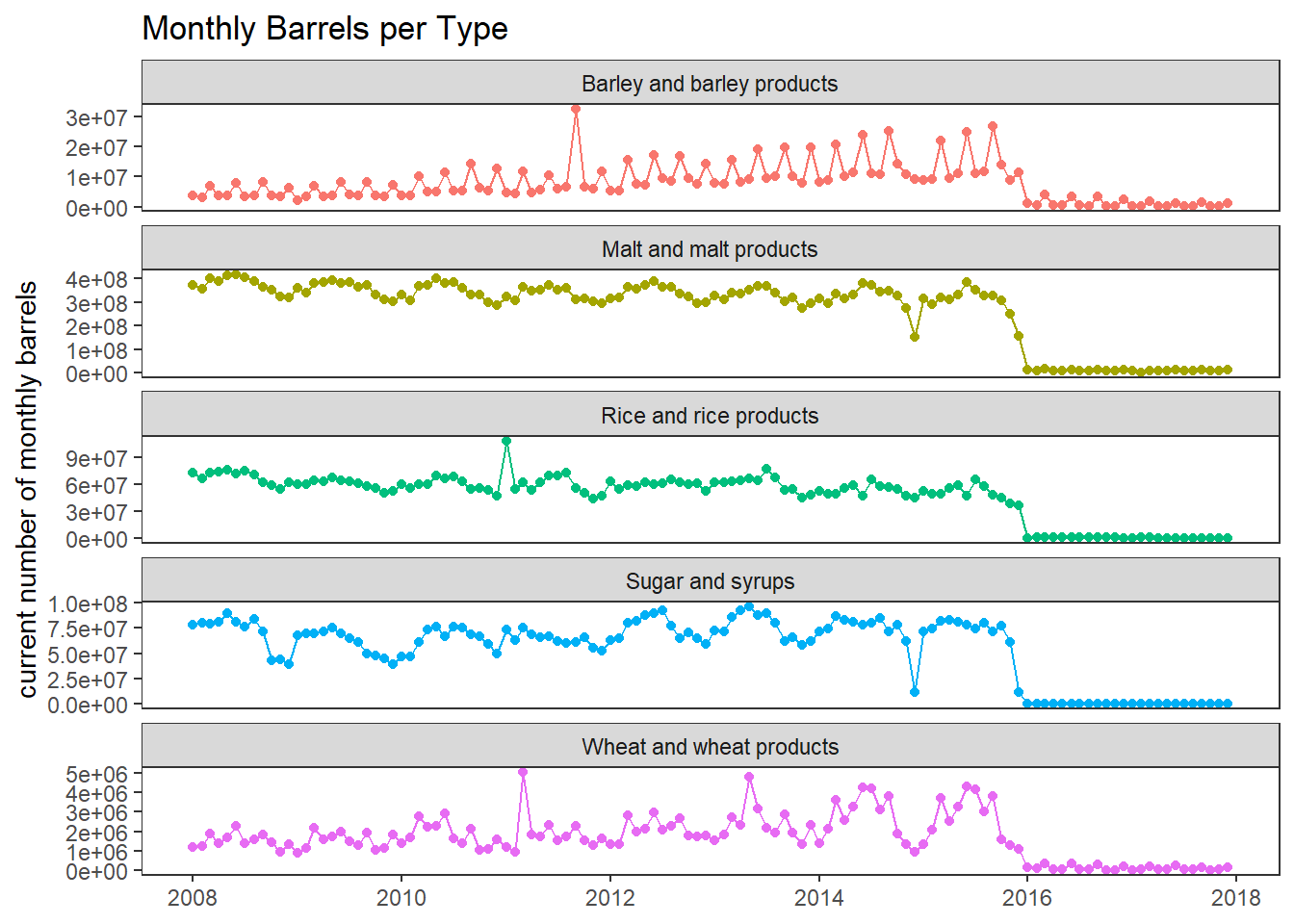
What happened after 2016? Why are the lines close to 0? I assume there is some data entry issue.
For the sake of our predictive modeling, data after year 2016 will be removed.
brew_before_2016 <- brewing_materials %>%
  filter(year < 2016)

brew_before_2016
## # A tibble: 480 x 5
## year month type month_prior_year month_current
## <dbl> <dbl> <chr> <dbl> <dbl>
## 1 2008 1 Malt and malt products 365300134 374165152
## 2 2008 1 Rice and rice products 81050102 72402143
## 3 2008 1 Barley and barley products 2362162 3800844
## 4 2008 1 Wheat and wheat products 1195381 1177186
## 5 2008 1 Sugar and syrups 83664091 78358212
## 6 2008 2 Malt and malt products 350035966 355687578
## 7 2008 2 Rice and rice products 75004651 66061597
## 8 2008 2 Barley and barley products 2573584 3236714
## 9 2008 2 Wheat and wheat products 1074183 1240983
## 10 2008 2 Sugar and syrups 86331629 80188744
## # ... with 470 more rowsbrew_before_2016 %>%
ggplot(aes(month_prior_year, month_current, color = type)) +
geom_point() +
scale_x_log10() +
scale_y_log10() +
labs(x = "monthly barrels prior year",
y = "monthly barrels current year",
title = "Monthly Barrels between Current and Prior Year")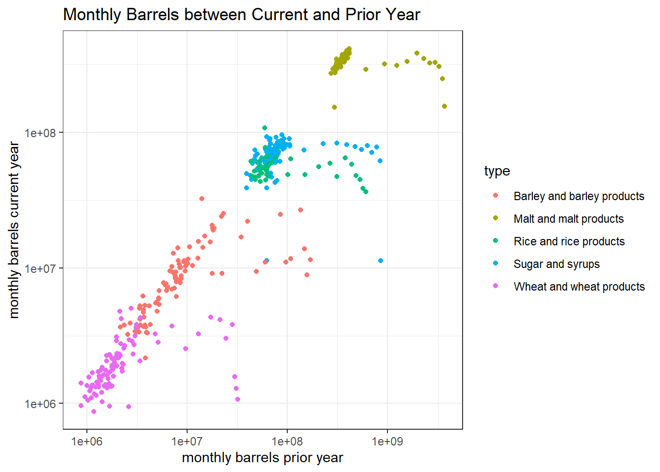
The relationship between current and prior monthly barrel is almost log-linear.
Below a LASSO model will be built to predict month_current.
- Split the data:
set.seed(2022)

brew_spl <- brew_before_2016 %>%
  initial_split(strata = "month")
brew_train <- training(brew_spl)
brew_test <- testing(brew_spl)

brew_boots <- bootstraps(brew_train, times = 1000, strata = "month")

brew_boots
## # Bootstrap sampling using stratification
## # A tibble: 1,000 x 2
## splits id
## <list> <chr>
## 1 <split [360/135]> Bootstrap0001
## 2 <split [360/132]> Bootstrap0002
## 3 <split [360/128]> Bootstrap0003
## 4 <split [360/128]> Bootstrap0004
## 5 <split [360/135]> Bootstrap0005
## 6 <split [360/144]> Bootstrap0006
## 7 <split [360/135]> Bootstrap0007
## 8 <split [360/139]> Bootstrap0008
## 9 <split [360/131]> Bootstrap0009
## 10 <split [360/132]> Bootstrap0010
## # ... with 990 more rows- Create the recipe:
brew_rec <- recipe(month_current ~ ., data = brew_train) %>%
  step_mutate(type = factor(type)) %>%
  step_log(month_prior_year, month_current, base = 10) %>%
step_dummy(all_nominal_predictors())- Set up the LASSO spec:
brew_spec <- linear_reg(penalty = tune(), mixture = 1) %>%
  set_mode("regression") %>%
set_engine("glmnet")- Set up the workflow:
brew_wf <- workflow() %>%
  add_model(brew_spec) %>%
add_recipe(brew_rec)- Tune the model:
brew_res <- brew_wf %>%
  tune_grid(
    brew_boots,
    grid = crossing(
      penalty = 10 ^ seq(-7, -0.5, 0.5)
    ),
    control = control_grid(save_pred = T,
                           save_workflow = T)
  )

autoplot(brew_res)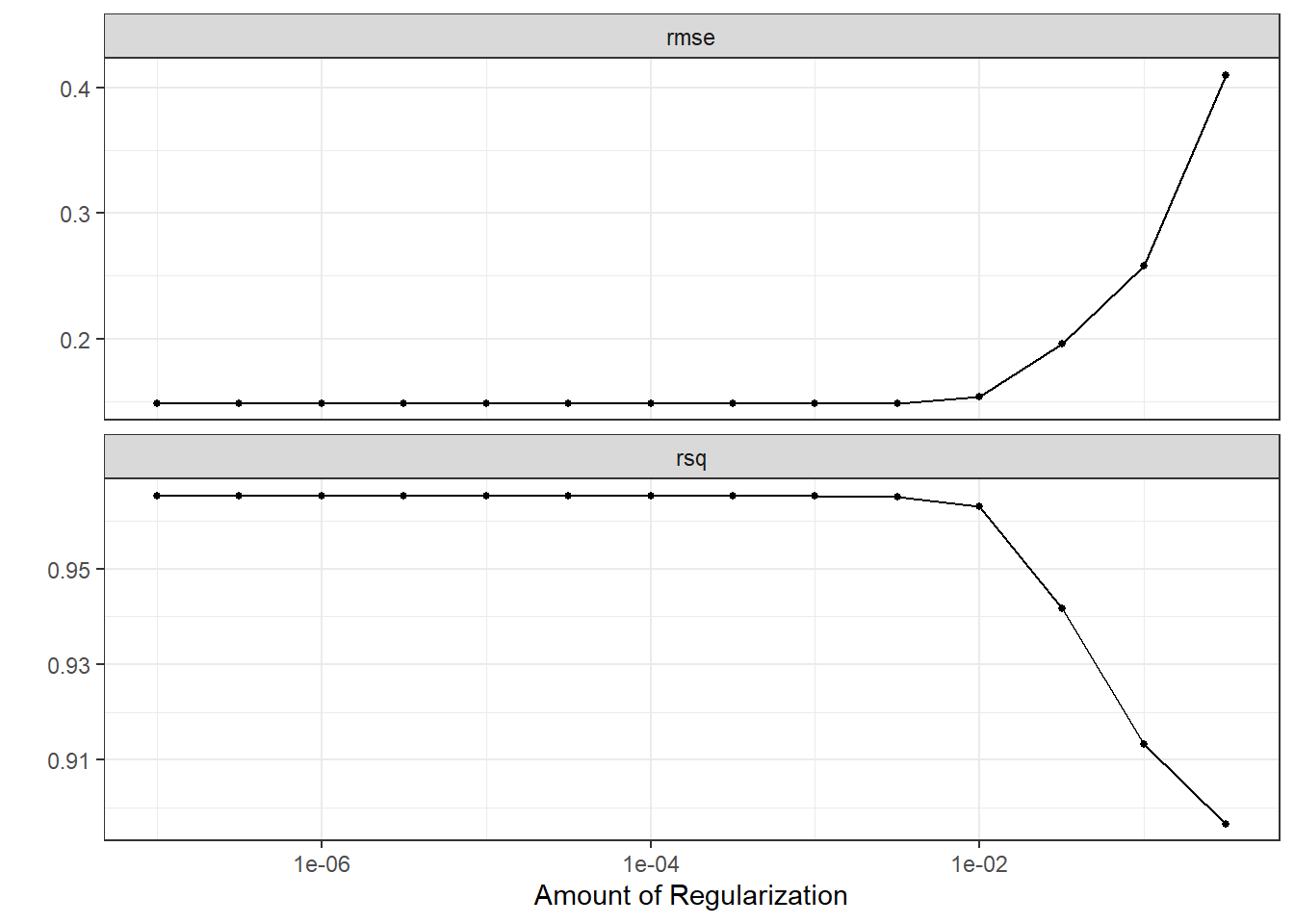
- Finalize the workflow:
brew_last_fit <- brew_wf %>%
  finalize_workflow(select_best(brew_res, "rmse")) %>%
  last_fit(brew_spl)

brew_last_fit %>%
  collect_metrics()
## # A tibble: 2 x 4
## .metric .estimator .estimate .config
## <chr> <chr> <dbl> <chr>
## 1 rmse standard 0.142 Preprocessor1_Model1
## 2 rsq standard 0.969 Preprocessor1_Model1brew_last_fit %>%
collect_predictions() %>%
ggplot(aes(month_current, .pred)) +
geom_point() +
geom_abline(size = 2, color = "grey50", lty = 2) 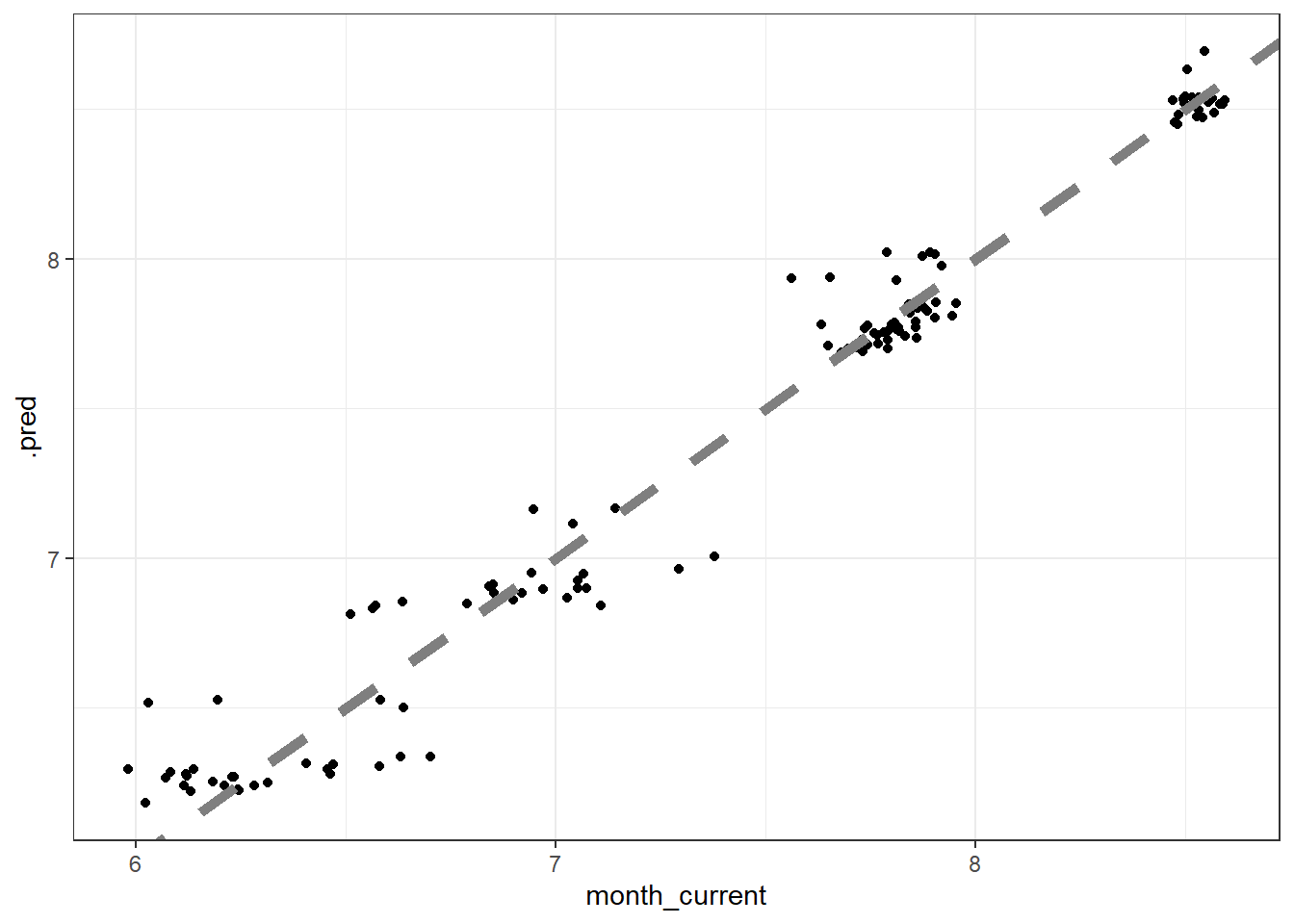
The LASSO does have a good prediction, but one thing to keep in mind is that the predictions are on log10 scale.