LASSO Model on Predicting GDPR Fines

Fri, May 27, 2022 4-minute read

In this blog post, I will use LASSO model to predict the GDPR fines. Before this post, I have another post on visualizing the same data set. You can view it here. Also, the textrecipes package is used in the modeling process, as the data set privodes some text columns, which can be transformed as predictors.

library(tidyverse)
library(lubridate)
library(tidymodels)
library(textrecipes)
theme_set(theme_bw())

gdpr_raw <- read_tsv("https://raw.githubusercontent.com/rfordatascience/tidytuesday/master/data/2020/2020-04-21/gdpr_violations.tsv") %>%
  mutate(date = mdy(date)) %>%
  select(-c(picture, source))

gdpr_raw

## # A tibble: 250 x 9
##       id name     price authority   date       controller article_violated type 
##    <dbl> <chr>    <dbl> <chr>       <date>     <chr>      <chr>            <chr>
##  1     1 Poland    9380 Polish Nat~ 2019-10-18 Polish Ma~ Art. 28 GDPR     Non-~
##  2     2 Romania   2500 Romanian N~ 2019-10-17 UTTIS IND~ Art. 12 GDPR|Ar~ Info~
##  3     3 Spain    60000 Spanish Da~ 2019-10-16 Xfera Mov~ Art. 5 GDPR|Art~ Non-~
##  4     4 Spain     8000 Spanish Da~ 2019-10-16 Iberdrola~ Art. 31 GDPR     Fail~
##  5     5 Romania 150000 Romanian N~ 2019-10-09 Raiffeise~ Art. 32 GDPR     Fail~
##  6     6 Romania  20000 Romanian N~ 2019-10-09 Vreau Cre~ Art. 32 GDPR|Ar~ Fail~
##  7     7 Greece  200000 Hellenic D~ 2019-10-07 Telecommu~ Art. 5 (1) c) G~ Fail~
##  8     8 Greece  200000 Hellenic D~ 2019-10-07 Telecommu~ Art. 21 (3) GDP~ Fail~
##  9     9 Spain    30000 Spanish Da~ 2019-10-01 Vueling A~ Art. 5 GDPR|Art~ Non-~
## 10    10 Romania   9000 Romanian N~ 2019-09-26 Inteligo ~ Art. 5 (1) a) G~ Non-~
## # ... with 240 more rows, and 1 more variable: summary <chr>

Clean up gdpr_raw:

gdpr <- gdpr_raw %>%
  filter(str_detect(article_violated, "Art\\."),
         price > 0) %>%
  mutate(article_violated = str_replace(article_violated, "\\.\\s", ""),
         article_violated = as.factor(as.integer(parse_number(article_violated))),
         authority = fct_lump(authority, n = 5),
         controller = fct_lump(controller, n = 8)) 

gdpr

## # A tibble: 236 x 9
##       id name     price authority   date       controller article_violated type 
##    <dbl> <chr>    <dbl> <fct>       <date>     <fct>      <fct>            <chr>
##  1     1 Poland    9380 Other       2019-10-18 Other      28               Non-~
##  2     2 Romania   2500 Romanian N~ 2019-10-17 Other      12               Info~
##  3     3 Spain    60000 Spanish Da~ 2019-10-16 Xfera Mov~ 5                Non-~
##  4     4 Spain     8000 Spanish Da~ 2019-10-16 Other      31               Fail~
##  5     5 Romania 150000 Romanian N~ 2019-10-09 Other      32               Fail~
##  6     6 Romania  20000 Romanian N~ 2019-10-09 Other      32               Fail~
##  7     7 Greece  200000 Other       2019-10-07 Other      5                Fail~
##  8     8 Greece  200000 Other       2019-10-07 Other      21               Fail~
##  9     9 Spain    30000 Spanish Da~ 2019-10-01 Other      5                Non-~
## 10    10 Romania   9000 Romanian N~ 2019-09-26 Other      5                Non-~
## # ... with 226 more rows, and 1 more variable: summary <chr>

GDPR fine price:

gdpr %>%
  ggplot(aes(price)) +
  geom_histogram() +
  scale_x_log10()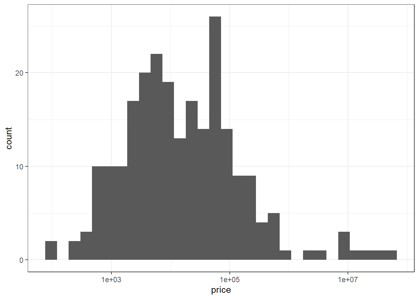

The price is sort of log-normal.

Now we can step in and begin to build up the model as following steps:

Data spending

set.seed(2022)
gdpr_spl <- gdpr %>%
  initial_split(strata = "price", prop = 0.8)

gdpr_train <- training(gdpr_spl)
gdpr_test <- testing(gdpr_spl)

gdpr_folds <- vfold_cv(gdpr_train, v = 20)

Data engineering

gdpr_rec <- recipe(price ~ ., data = gdpr_train) %>%
  update_role(id, new_role = "id") %>%
  step_other(name, article_violated) %>%
  step_date(date, features = c("year", "month")) %>%
  step_rm(date) %>%
  step_tokenize(type, summary) %>%
  step_stopwords(type, summary) %>%
  step_tokenfilter(type, max_tokens = 3) %>%
  step_tokenfilter(summary, max_tokens = 5) %>%
  step_tfidf(type, summary) %>%
  step_dummy(all_nominal_predictors()) %>%
  step_nzv(all_predictors()) %>%
  step_log(price, base = 10)

Model sepcification

We use LASSO to predict the price:

lasso_spec <- linear_reg(penalty = tune()) %>%
  set_mode("regression") %>%
  set_engine("glmnet")

LASSO workflow

lasso_wf <- workflow() %>%
  add_model(lasso_spec) %>%
  add_recipe(gdpr_rec)

Model Tuning

lasso_res <- lasso_wf %>%
  tune_grid(
    gdpr_folds,
    grid = crossing(penalty = 10 ^ seq(-7, -0.1, 0.1)),
    control = control_grid(save_pred = T,
                           save_workflow = T)
  )

autoplot(lasso_res)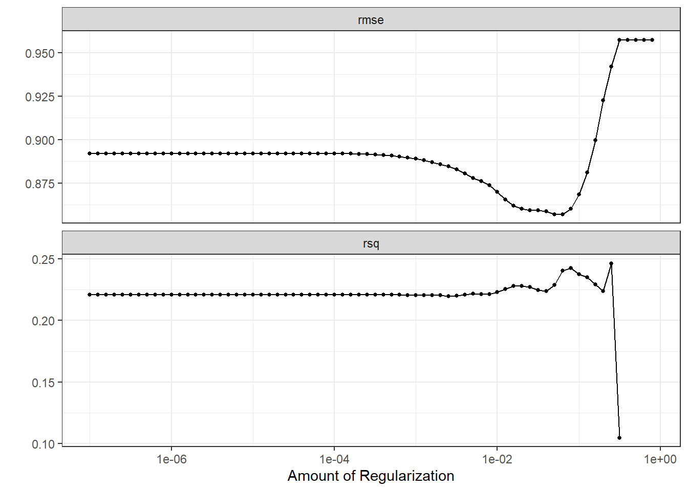

The R squared is surprisingly low, meaning that the model doesn’t explain the data variation well.

Finalize the workflow and train the last time:

lasso_last_fit <- lasso_wf %>%
  finalize_workflow(select_best(lasso_res, "rmse")) %>%
  last_fit(gdpr_spl)

lasso_last_fit %>%
  collect_metrics()

## # A tibble: 2 x 4
##   .metric .estimator .estimate .config             
##   <chr>   <chr>          <dbl> <chr>               
## 1 rmse    standard       0.946 Preprocessor1_Model1
## 2 rsq     standard       0.102 Preprocessor1_Model1

lasso_last_fit %>%
  collect_predictions() %>%
  ggplot(aes(price, .pred)) +
  geom_point() +
  geom_abline() +
  labs(x = "price (log)",
       y = ".pred (log)",
       title = "Price VS Prediction")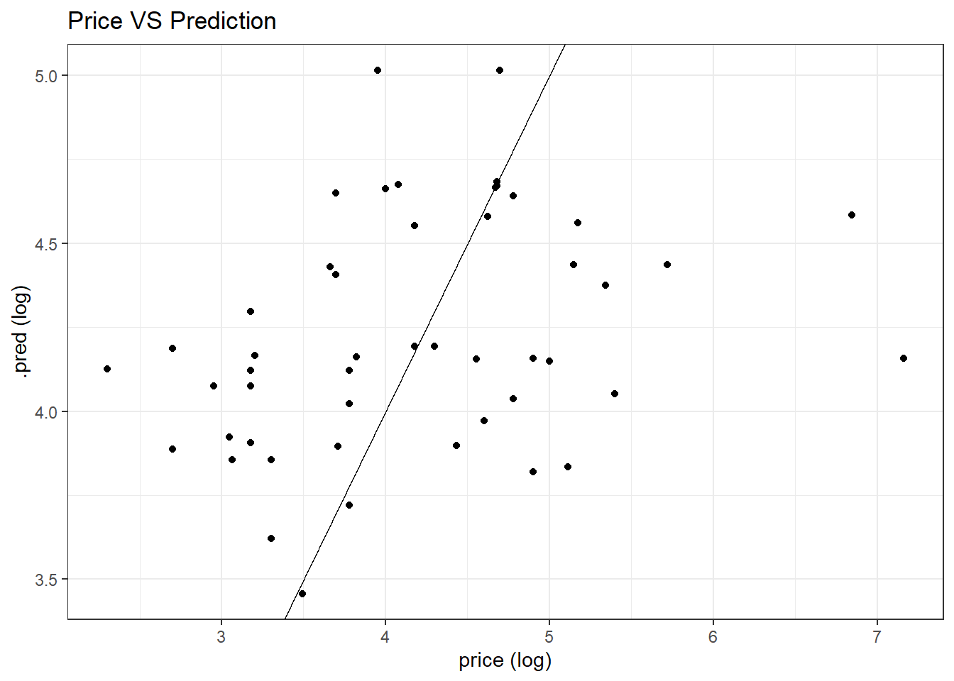

As we can see, LASSO does not fit the data well, as the predictions are spread-out. Maybe because there is some outliers making the predictions difficult. But through this model training and testing process, some light is shed on how to use the tidymodels metapackage and textrecipes to make model prediction.