Using LASSO Bootstraps to Predict Animal Crossing Rating

In this blog post, I will use the tidymodels meta-package to predict the animal crossing rating. Previously, I had a blog post visualizing the same data set, and you can view it here. Since the data set contains user comments along with the game rating, and LASSO is a good model for using words as predictors, this blog post I will use bootstrap resampling method to illustrate how to tune the LASSO model and # of words as predictors in the feature engineering steps. It is also worth noting that a few ideas (e.g., bootstrapping) are inspired by Julia Silge’s blog post on analyzing the same data set (link).

library(tidyverse)
library(tidymodels)
library(textrecipes)
theme_set(theme_bw())

user_reviews <- read_tsv("https://raw.githubusercontent.com/rfordatascience/tidytuesday/master/data/2020/2020-05-05/user_reviews.tsv") %>%
  rename(rating = grade)

user_reviews

## # A tibble: 2,999 × 4
##    rating user_name    text                                           date      
##     <dbl> <chr>        <chr>                                          <date>    
##  1      4 mds27272     My gf started playing before me. No option to… 2020-03-20
##  2      5 lolo2178     While the game itself is great, really relaxi… 2020-03-20
##  3      0 Roachant     My wife and I were looking forward to playing… 2020-03-20
##  4      0 Houndf       We need equal values and opportunities for al… 2020-03-20
##  5      0 ProfessorFox BEWARE!  If you have multiple people in your … 2020-03-20
##  6      0 tb726        The limitation of one island per Switch (not … 2020-03-20
##  7      0 Outryder86   I was very excited for this new installment o… 2020-03-20
##  8      0 Subby89      It's 2020 and for some reason Nintendo has de… 2020-03-20
##  9      0 RocketRon    This is so annoying. Only one player has the … 2020-03-20
## 10      0 chankills    I purchased this game for my household (me an… 2020-03-20
## # … with 2,989 more rows

EDA:

user_reviews %>%
  ggplot(aes(date)) +
  geom_histogram() +
  theme(panel.grid = element_blank()) +
  labs(title = "Date Distribution")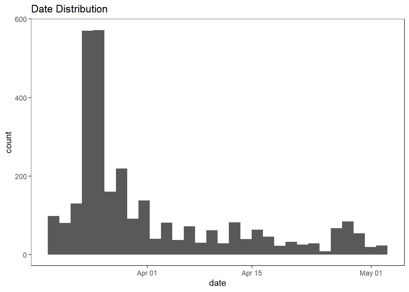

user_reviews %>%
  ggplot(aes(rating)) +
  geom_histogram(fill = "purple") +
  scale_x_continuous(breaks = seq(0, 10)) +
  theme(panel.grid = element_blank()) +
  labs(title = "Rating Distribution")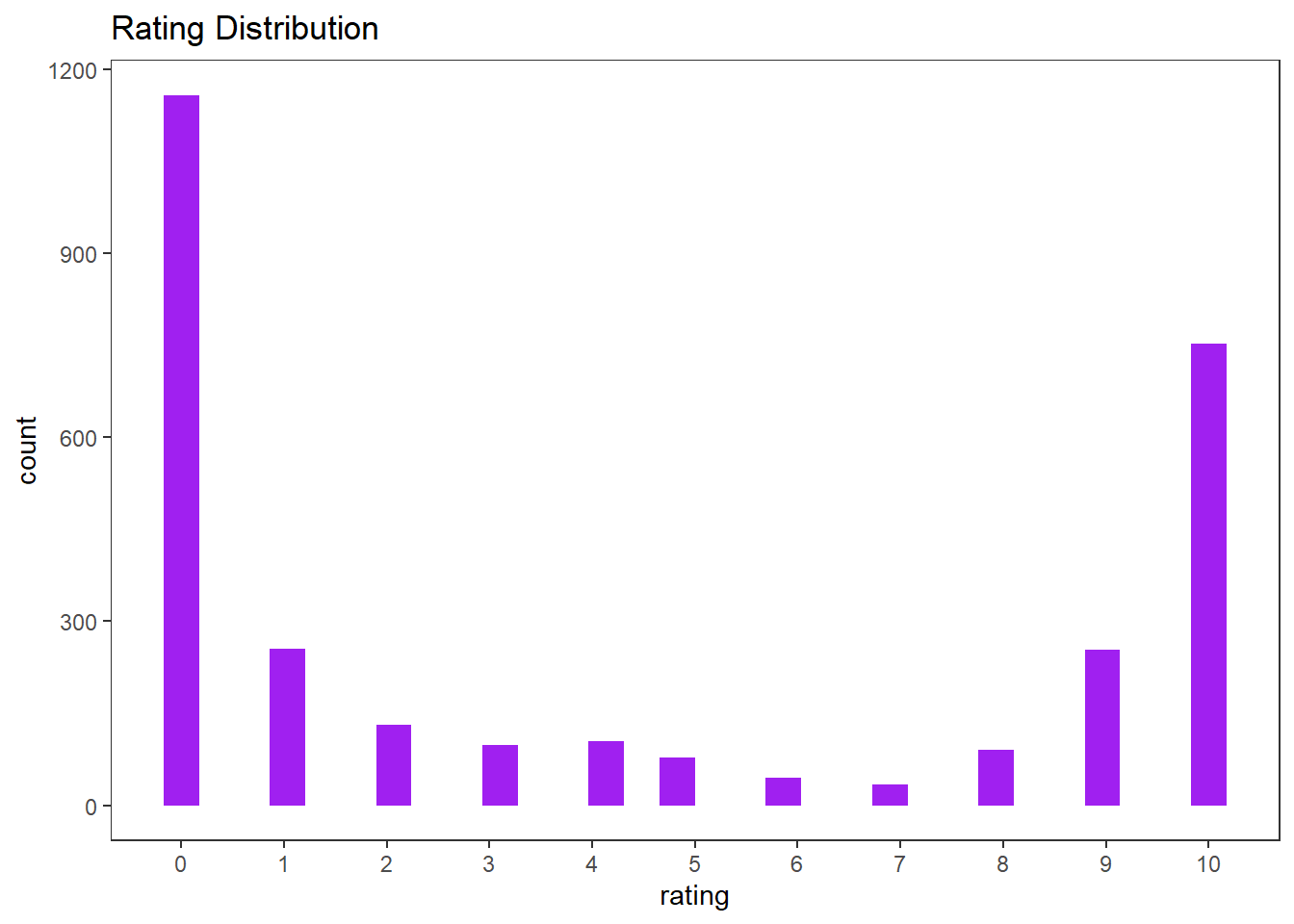

Model Building

• Data split

set.seed(2022)
review_spl <- user_reviews %>%
  initial_split(strata = "rating")

review_train <- training(review_spl) 
review_test <- testing(review_spl)

review_boot <- bootstraps(review_train, times = 100, strata = "rating")

• Feature engineering

review_rec <- recipe(rating ~ ., data = review_train) %>%
  update_role(user_name, new_role = "id") %>%
  step_date(date, features = "month") %>%
  step_rm(date) %>%
  step_tokenize(text) %>%
  step_stopwords(text) %>%
  step_tokenfilter(text, max_tokens = tune()) %>%
  step_tf(text) %>%
  step_dummy(all_nominal_predictors())

• Model specification and workflow

lasso_spec <- linear_reg(penalty = tune()) %>%
  set_mode("regression") %>%
  set_engine("glmnet")

lasso_wf <- workflow() %>%
  add_model(lasso_spec) %>%
  add_recipe(review_rec)

• Model tuning

lasso_res <- lasso_wf %>%
  tune_grid(
    review_boot,
    grid = crossing(
      max_tokens = c(50, 100, 150, 200, 300, 500),
      penalty = 10 ^ seq(-7, -0.5, 0.5)
    )
  )

autoplot(lasso_res)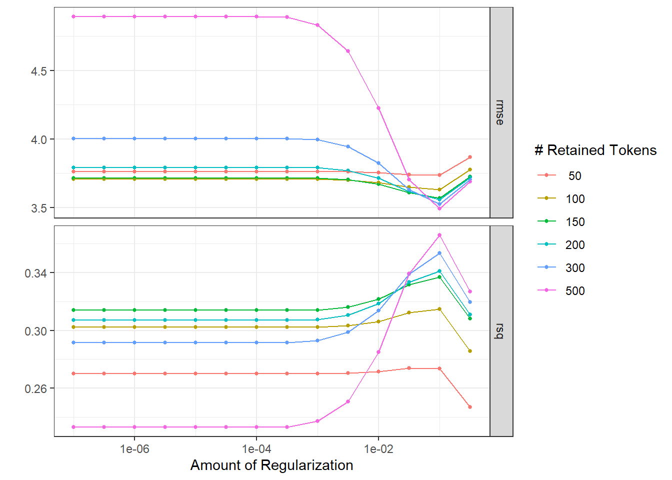

lasso_res %>%
  show_best()

## # A tibble: 5 × 8
##   penalty max_tokens .metric .estimator  mean     n std_err .config             
##     <dbl>      <dbl> <chr>   <chr>      <dbl> <int>   <dbl> <chr>               
## 1  0.1           500 rmse    standard    3.49   100 0.00462 Preprocessor6_Model…
## 2  0.1           300 rmse    standard    3.53   100 0.00498 Preprocessor5_Model…
## 3  0.1           200 rmse    standard    3.56   100 0.00460 Preprocessor4_Model…
## 4  0.1           150 rmse    standard    3.57   100 0.00476 Preprocessor3_Model…
## 5  0.0316        150 rmse    standard    3.61   100 0.00622 Preprocessor3_Model…

• Finalize the workflow

lasso_last_fit <- lasso_wf %>%
  finalize_workflow(lasso_res %>%
                      select_best("rmse")) %>%
  last_fit(review_spl)

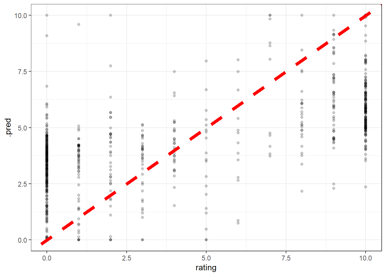
lasso_last_fit %>%
  collect_predictions() %>%
  ggplot(aes(rating, .pred)) +
  geom_point(alpha = 0.2) +
  geom_abline(lty = 2, color = "red", size = 2)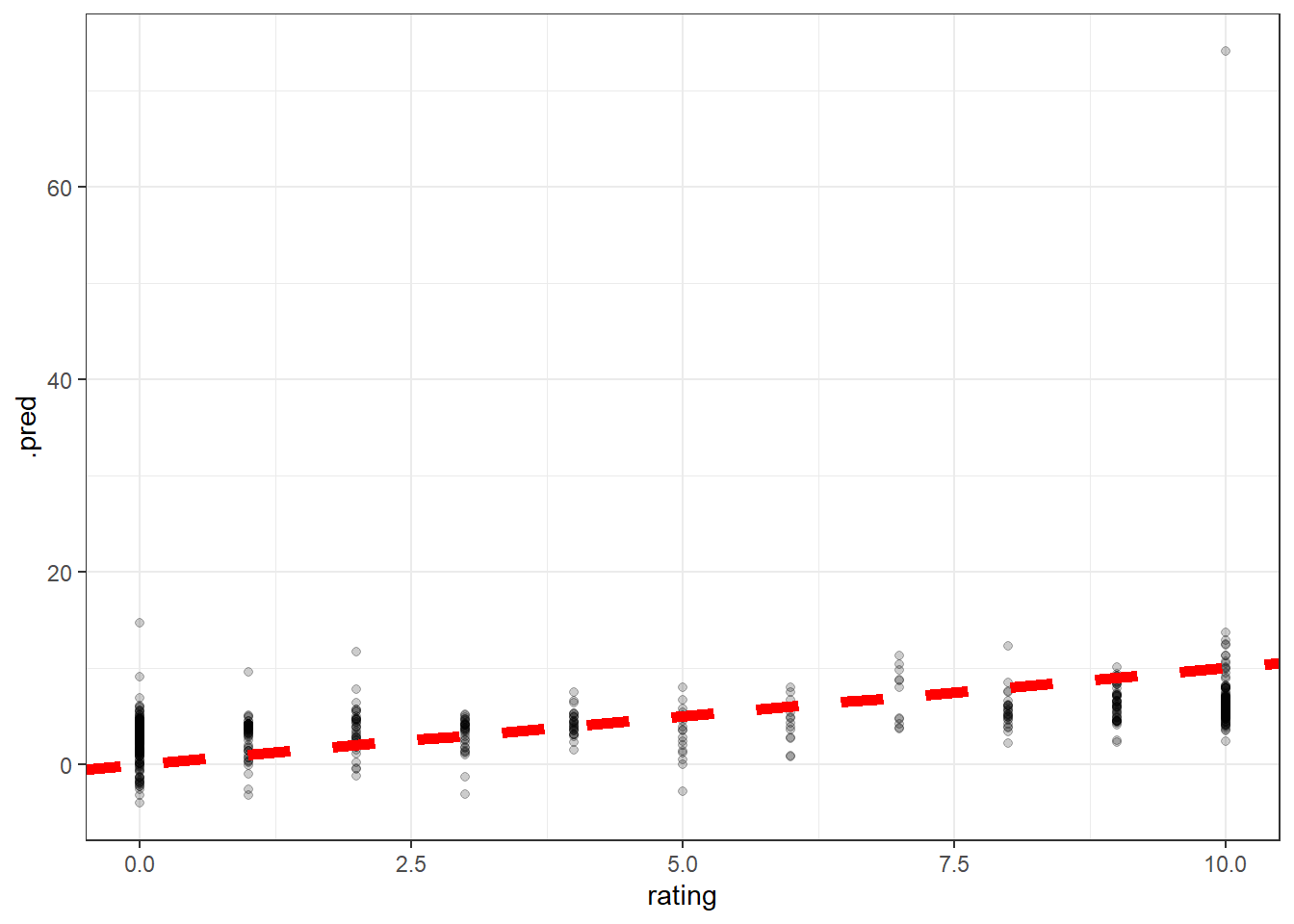

For some reason, thre is a prediction that is much larger than usual.

We can transform the prediction in a way that if the value is greater than 10 or less than 0, set it as 10 or 0.

lasso_last_fit %>%
  collect_metrics()

## # A tibble: 2 × 4
##   .metric .estimator .estimate .config             
##   <chr>   <chr>          <dbl> <chr>               
## 1 rmse    standard       4.14  Preprocessor1_Model1
## 2 rsq     standard       0.206 Preprocessor1_Model1

lasso_fit_refined <- lasso_last_fit %>%
  collect_predictions() %>%
  mutate(.pred = case_when(.pred > 10 ~ 10,
                           .pred < 0 ~ 0,
                           TRUE ~ .pred)) 

lasso_fit_refined %>%
  rmse(rating, .pred) 

## # A tibble: 1 × 3
##   .metric .estimator .estimate
##   <chr>   <chr>          <dbl>
## 1 rmse    standard        3.33

We can see there is great improvement on RMSE. Now let’s plot the new predictions.

lasso_fit_refined %>%
  ggplot(aes(rating, .pred)) +
  geom_point(alpha = 0.2) +
  geom_abline(lty = 2, color = "red", size = 2)