A Desktop Grace Blackwell Machine as Research Infrastructure: Serving and Training Benchmarks for the NVIDIA DGX Spark
Contents 7 sections
The NVIDIA DGX Spark is a desktop computer containing a GB10 Grace Blackwell system on a chip: one GPU with 48 streaming multiprocessors, twenty ARM cores, and 121.7 GiB of LPDDR5X memory that the processor and the accelerator share as a single pool. It draws under one hundred watts. It is, in other words, an unremarkable-looking box that happens to hold more addressable accelerator memory than an eighty-gigabyte H100.
Two questions follow from that, and this article answers both with measurements. The first is whether such a machine can serve a modern language model well enough to host a real application. The second is whether it can train one, and how its throughput compares with the datacenter accelerators that normally do that work.
The answers are not the same, and the difference between them is the most useful thing here. The Spark reaches roughly ten per cent of an H200 when training, and roughly forty per cent when generating tokens, because those two activities are limited by different resources. Understanding why is worth more than either number alone.
What the machine actually is
Two figures bound everything that follows: how much arithmetic the card can perform, and how quickly it can move data. Both were measured directly, with the same script running in the same process on every card, rather than taken from a specification sheet.
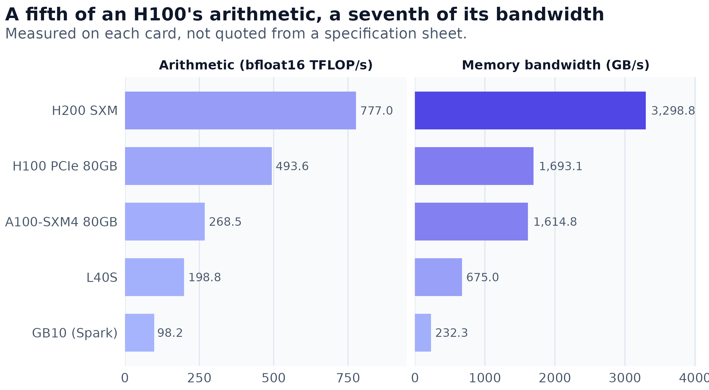
Figure 1: Measured dense arithmetic throughput and memory bandwidth for five accelerators. Each value is a square matrix multiplication at n = 8192 and a device-to-device copy, run by the same script on each card. The H100 PCIe figure is the mean of four separate process starts, which ranged from 477.4 to 516.3, or 7.9 per cent of that mean; the H200 figure is the mean of three, which ranged over 2.3 per cent.
Relative to an H200, the Spark holds 12.6 per cent of the arithmetic and 7.0 per cent of the bandwidth. Those two fractions bracket every performance number in this article. Work dominated by matrix multiplication lands near the first; work dominated by moving weights lands near the second.
The third number is capacity, and it runs the other way. The Spark’s 121.7 GiB is more than an H100 or an A100 holds, and unlike theirs it is shared with the operating system rather than separate from host memory. That single design decision is responsible for both the machine’s most interesting capability and its most dangerous failure mode, and both appear later.
Part I: Serving an agentic assistant
The application that motivated this work is Sage, a documentation assistant for the University of Chicago’s Research Computing Center. A user asks a question in natural language; the assistant searches a corpus of the centre’s user guide, reads the pages it finds, and answers with citations back to them. It is agentic in the specific sense that the model decides what to search for and when it has read enough, calling tools in a loop rather than receiving a fixed context.
Sage normally runs against a hosted commercial model. The deployment measured here replaces that with a model running on the Spark itself: same corpus, same retrieval, same interface, same citations, but every token generated on a desk rather than in someone else’s datacenter. The corpus and the questions never leave the building.
The model is NVIDIA Nemotron-3.5-Lightning-30B-A3B, quantised to NVFP4. It has thirty billion parameters in total but activates only about three billion for any given token, because it is a mixture of experts: a routing layer selects a small subset of the available parameters per token. Quantised to four bits it occupies twenty-one gigabytes on disk. It is served by vLLM 0.27.1 with multi-token prediction enabled, and a small proxy in front of it gives the application a fixed address so the engine underneath can be restarted without the app noticing.
Generation speed
The headline figure is 106.3 tokens per second for a single stream with greedy decoding. Under sampling, which is what the application actually uses, the rate is slightly lower and declines gently as the answer grows longer.
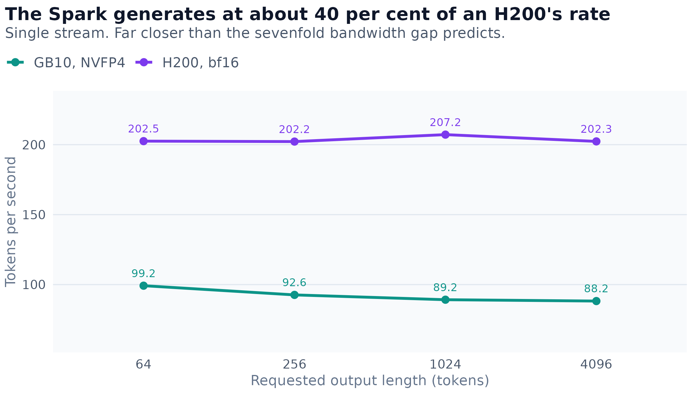
Figure 2: Token generation rate against the length of the requested output, for the same model on the Spark at four-bit precision and on an H200 at sixteen-bit precision. Direct labels give the rate in tokens per second. The Spark’s decline across the range is 11 per cent; the H200’s rate is flat. The H200 is the only datacenter card the serving suite was run on, and it is the fastest of the three measured for training, so this and the following serving comparisons are the least favourable ones available to the Spark rather than the most.
Two ratios are worth separating here. The figure compares each machine as it is actually configured, and the Spark lands at 43 to 49 per cent. Holding the algorithm constant by disabling the Spark’s speculative decoding, which the H200 configuration does not use, gives 38.6 per cent, and that is the figure used later when comparing phases.
Either way it is a much better showing than the 7.0 per cent bandwidth ratio predicts, and the reason is precision. Generating a token requires reading the active weights out of memory, and four-bit weights are a quarter of the bytes of sixteen-bit ones. A card starved of bandwidth therefore gains far more from quantisation than a card with bandwidth to spare. Seven per cent of the bandwidth multiplied by four times fewer bytes per token is 28 per cent, and the remainder is accounted for by which parameters a mixture-of-experts model actually reads.
The number that matters to a reader, and it is not the first one
Nemotron-3.5-Lightning is a reasoning model. Before it answers, it writes out a chain of thought, and the serving stack streams that trace separately from the answer. This makes “time to first token” ambiguous in a way that matters.
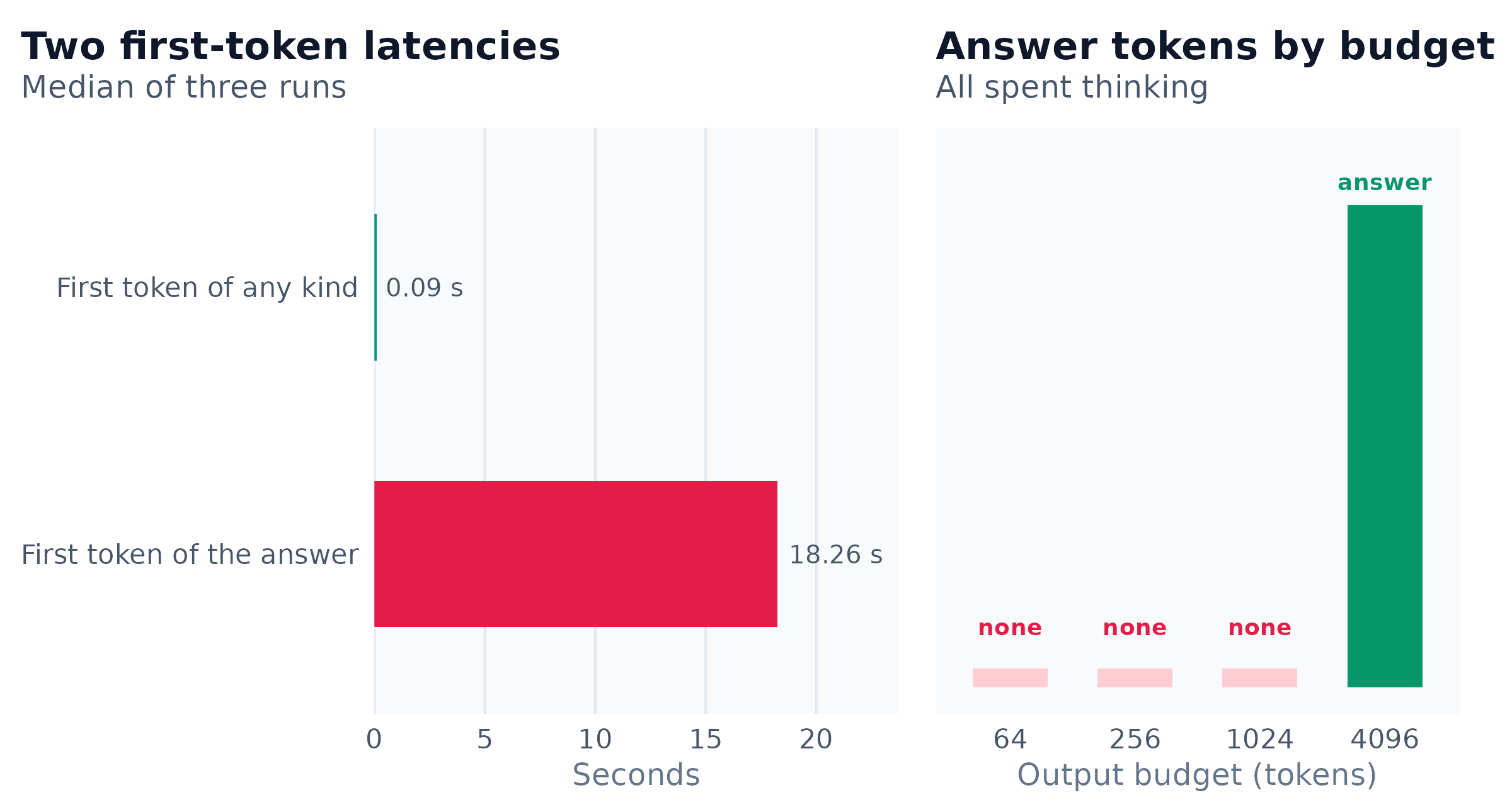
Figure 3: Two latencies on the same request. Time to first token is what a monitoring dashboard records; time to the first token of the answer is what a reader waits for. The right panel gives the number of answer tokens produced under four output budgets, three runs each.
A monitoring dashboard watching this deployment would report a 97-millisecond time to first token and conclude the service is fast. A reader waits eighteen seconds. On one measured 2,465-token answer the first visible word arrived at 23.29 seconds of a 25.09-second turn: ninety-three per cent of the wall clock was deliberation.
The consequence for anyone deploying this class of model is sharper than a latency figure. At output budgets of 64, 256 and 1,024 tokens the model produced no answer tokens at all, three runs each. The reasoning consumed the entire allowance and the stream was cut off mid-thought. The deployment sets a budget of twelve thousand tokens, which had looked generous and is in fact close to the minimum that works. A reasonable-seeming cap of 512 or 1,024 tokens would make this model appear broken.
The application conceals the wait by streaming the reasoning trace to the reader, which is why it feels responsive despite the underlying number.
Smoothness
Average generation rate says nothing about whether a stream stutters. The distribution of gaps between tokens does.
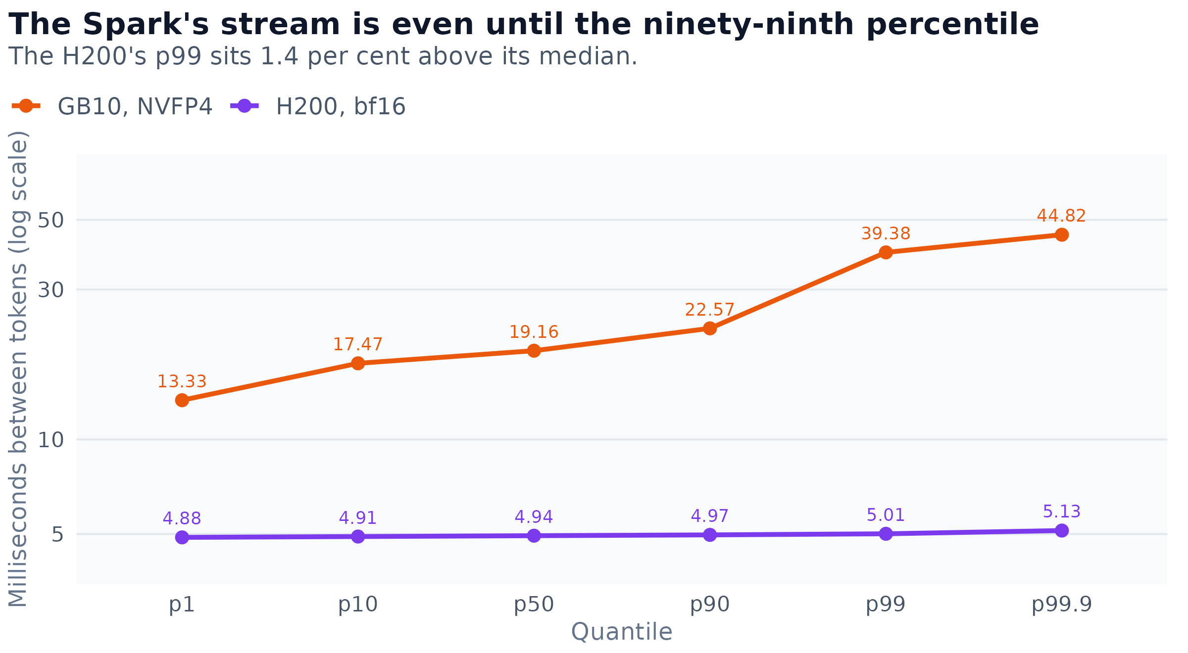
Figure 4: Distribution of the interval between consecutive tokens, pooled over 1,670 gaps on the Spark and 2,046 on the H200. Note the logarithmic vertical axis. The Spark’s ninety-ninth percentile is almost exactly twice its median, which is the cost of one rejected speculation.
The Spark’s stream is smooth in ordinary operation: the ninetieth percentile sits eighteen per cent above the median. The tail is a single phenomenon rather than general jitter, and identifying it required a separate experiment described below. The H200’s ratio of 1.014 between ninety-ninth percentile and median is what a card with three terabytes per second of bandwidth looks like when it never has to guess.
Reading a long document
Prefill is the phase that processes the prompt before generation begins. Its throughput rises with prompt length as the hardware fills, then falls as attention’s quadratic term takes over.
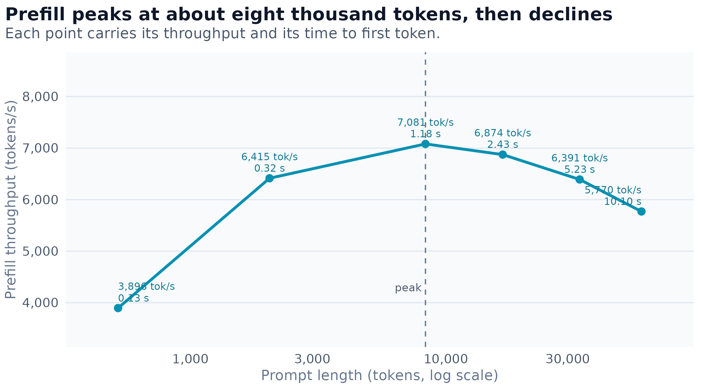
Figure 5: Prefill throughput and the resulting wait for the first token, against prompt length, on cold prompts with no cache reuse. The vertical marker is the point of peak throughput. Beyond it the rate declines because attention cost grows with the square of the sequence length while the key-value cache is written through 232 GB/s.
A fifty-eight-thousand-token prompt takes ten seconds before the first token appears. This is the Spark’s weakest phase relative to a datacenter card, at 16.6 per cent of an H200, because prefill is compute-bound and compute is where the gap is widest.
Long context is nearly free after that
Conventional attention keeps a key-value cache that grows with the sequence, and reading it back dominates generation once the context is long. This model is a hybrid: most of its layers carry a fixed-size recurrent state instead.
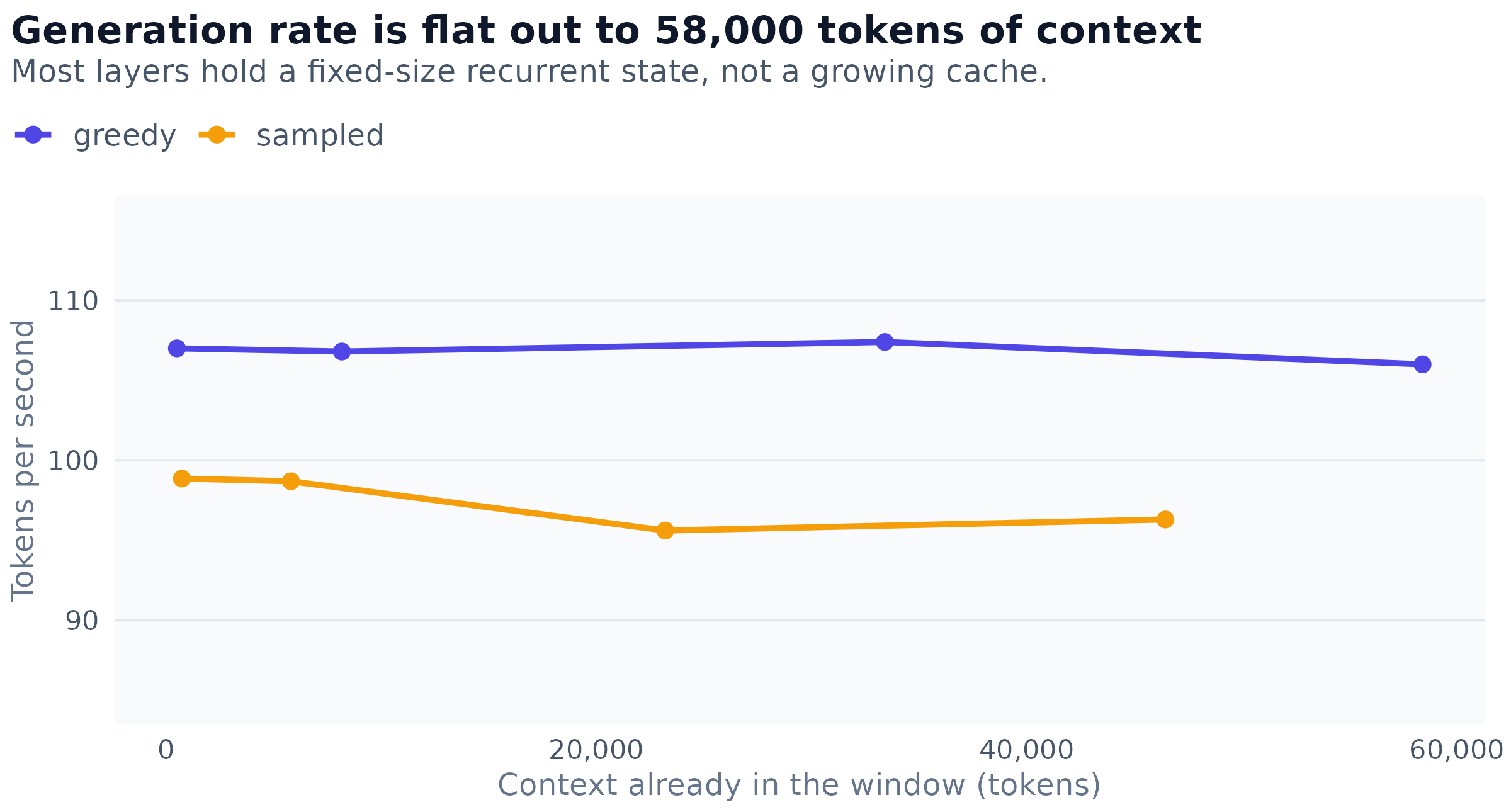
Figure 6: Token generation rate against how much context is already in the window, from two independent runs using different samplers and different prompt sets. Both are flat. On a conventional attention-only model of this size the rate would visibly decline as the cache grew.
Across a hundred-fold increase in context the greedy run varies by 1.3 per cent and the sampled run by 3.3 per cent. For a retrieval application this is the single most useful property of the architecture: adding more retrieved material to a prompt costs prefill once and does not slow the answer down.
What speculative decoding is actually worth
The engine runs multi-token prediction, a form of speculative decoding in which a small draft head proposes the next token and the main model verifies it. The published acceptance rate is 97.6 per cent and each engine step emits 1.96 tokens, from which it is tempting to conclude that generation is nearly twice as fast as it would otherwise be.
That conclusion is wrong, and establishing so required running a second engine on the same machine with the same weights and the same flags, varying only the speculation depth.
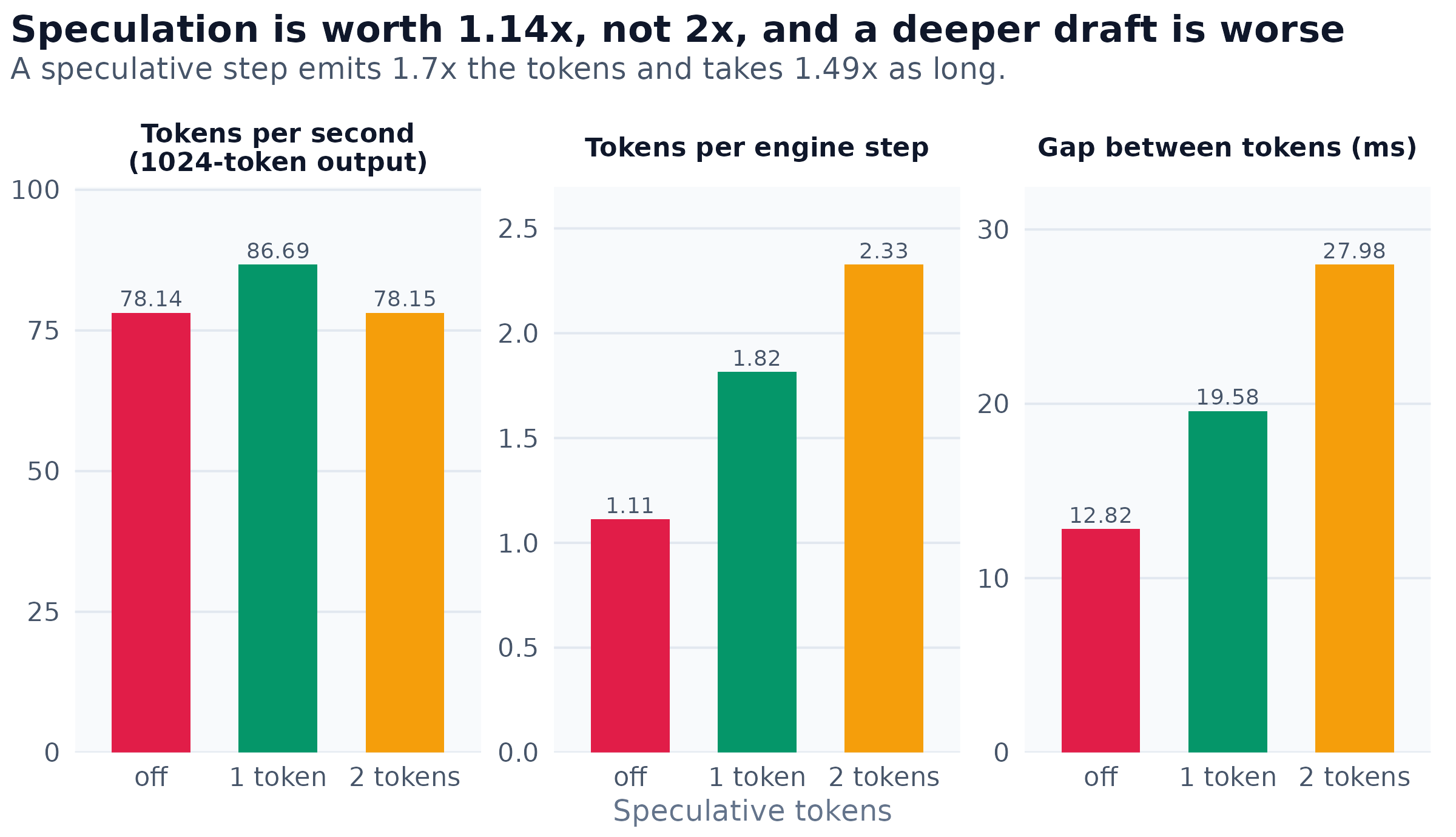
Figure 7: Speculative decoding depth against three measures, from a second engine instance differing from the deployed one only in this setting. Tokens per engine step rise with depth while the time each step takes rises faster, so throughput peaks at a depth of one.
Measured directly, speculation is worth between 1.14 and 1.19 times, not two. The mechanism is visible in the third panel: a speculative step emits 1.7 times the tokens but takes 1.49 times as long, because it must run the draft head and then verify its proposal. Net throughput is the ratio of those two effects, and only one of them appears in an acceptance rate.
Going to a depth of two makes matters worse. The second draft token is accepted only sixty-six per cent of the time against the first token’s eighty-two per cent, and it is paid for on every step regardless. At a thousand-token output, depth two is indistinguishable from no speculation at all. The shipped default of one is correct.
One consolation for the deeper setting is worth noting: it produces by far the most even stream, with a ninety-ninth percentile only 1.12 times its median, because step time comes to be dominated by the fixed cost of drafting and verifying rather than by whether a guess landed.
How many people can use it at once
The deployed engine reserves a quarter of the memory pool and eight concurrent request slots, deliberately, so that other work can share the machine. Both are policy rather than hardware limits, so a second configuration gave the engine ninety per cent of the pool and thirty-two slots.
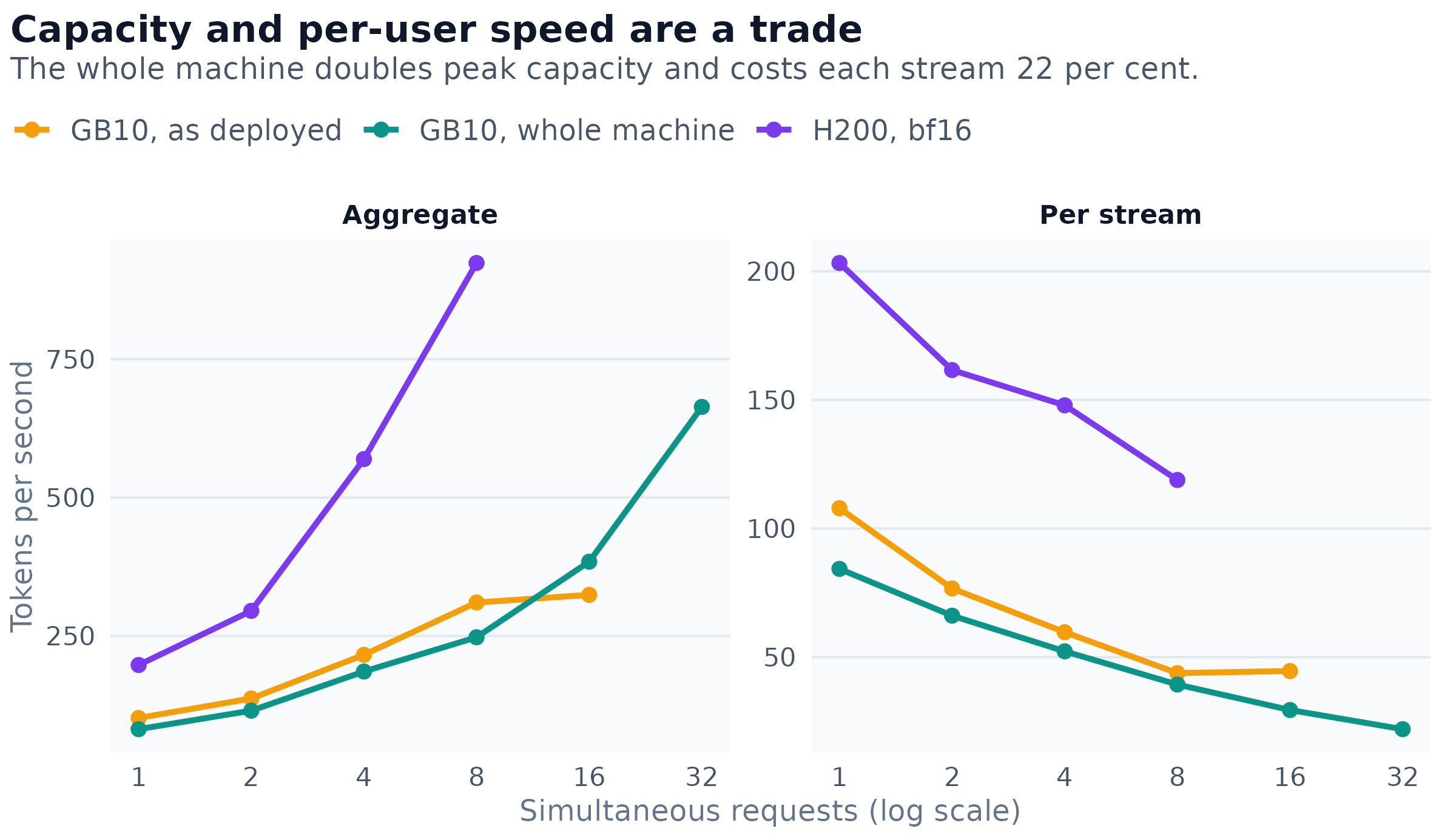
Figure 8: Aggregate and per-stream generation rate against the number of simultaneous requests, for two Spark configurations and the same model on an H200. The deployed configuration saturates at eight slots: its sixteen-stream point gains four per cent of throughput and its median wait rises to 3.41 seconds because the ninth request queues.
Giving the engine the whole machine raises peak aggregate throughput from 324 to 664 tokens per second, and the deployed configuration only reached its ceiling by queueing: at sixteen streams its median wait was 3.41 seconds, against 0.388 seconds for the larger configuration carrying twice the load. But single-stream generation falls from 107.9 to 84.3 tokens per second, and the ninety-ninth-percentile gap between tokens degrades 4.6 times across the range.
The rule that follows is simple. Choose the small configuration for a handful of users who each want a fast answer, and the large one for many users who will tolerate twenty-two tokens per second each.
Whether the answers are any good
Speed is worthless if the assistant is wrong. The application ships an evaluation harness with a labelled question bank, and it was run against this deployment: 116 tool-driven turns, scored for whether the assistant answered, whether it searched first, whether it cited the correct page, and whether it correctly declined questions the corpus cannot answer.
The same 116 turns were then run against the same checkpoint at sixteen-bit precision on an H200, which isolates what four-bit quantisation costs.
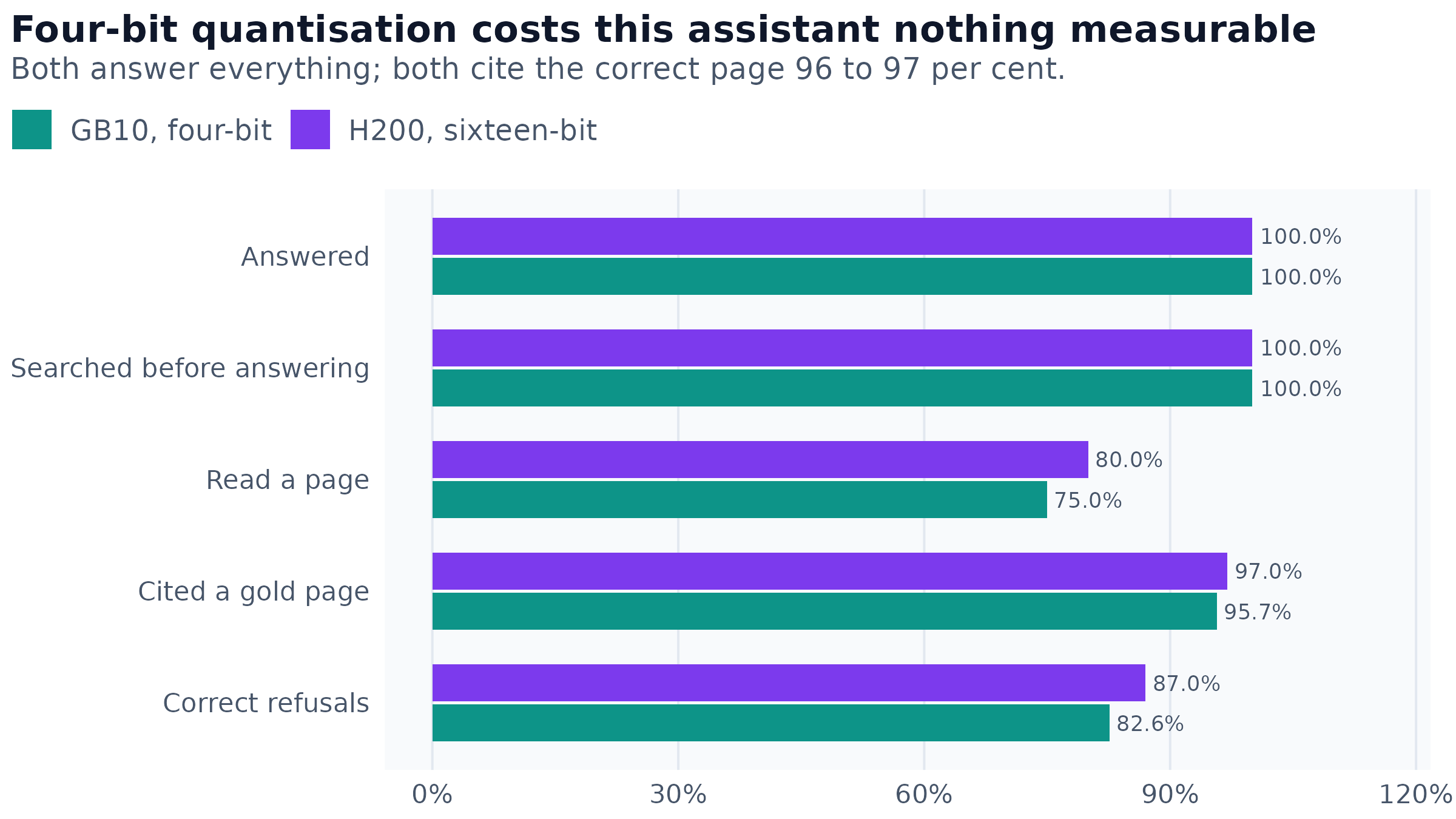
Figure 9: Agentic evaluation over 116 tool-driven turns, comparing the four-bit deployment against the same checkpoint at sixteen-bit precision on identical questions. Higher is better throughout. Tool calls never malformed in either run.
Both configurations answered every question, always searched before answering, and never emitted a malformed tool call in 116 turns. The four-bit deployment cited the correct page 95.7 per cent of the time against 97.0, and refused correctly 82.6 per cent of the time against 87.0: differences of roughly one and two turns respectively. Defects per answer were 0.11 for four-bit against 0.23 for sixteen-bit, which favours the quantised run, but that difference rests on a single small-count category and the two runs also differ in engine version, so the defensible conclusion is the null one. Quantisation does not measurably degrade this assistant.
The assistant’s genuine weakness lies elsewhere. Eight of its thirteen defects are a single class: answering a question it should have declined. That is the direct cost of a prompt rule introduced to fix the opposite failure, in which the model declined without searching. One rule, two failure modes, and it trades between them.
What the agentic machinery costs
Every turn of this application carries tool schemas, which engages the serving engine’s guided decoding path: a grammar compiled for the request and a mask applied to the model’s output at every step. This is overhead that a plain generation benchmark never sees.
Measured on identical prompts, attaching tool schemas costs fifty-seven milliseconds of time to first token and nothing measurable afterwards: generation rate and inter-token latency are unchanged within noise. At the 4.6 tool rounds the assistant averages per turn, that is about 0.26 seconds of a 10.4-second turn, under three per cent. A forced JSON output schema costs nothing at all.
Where a turn’s time goes, and what it costs to run
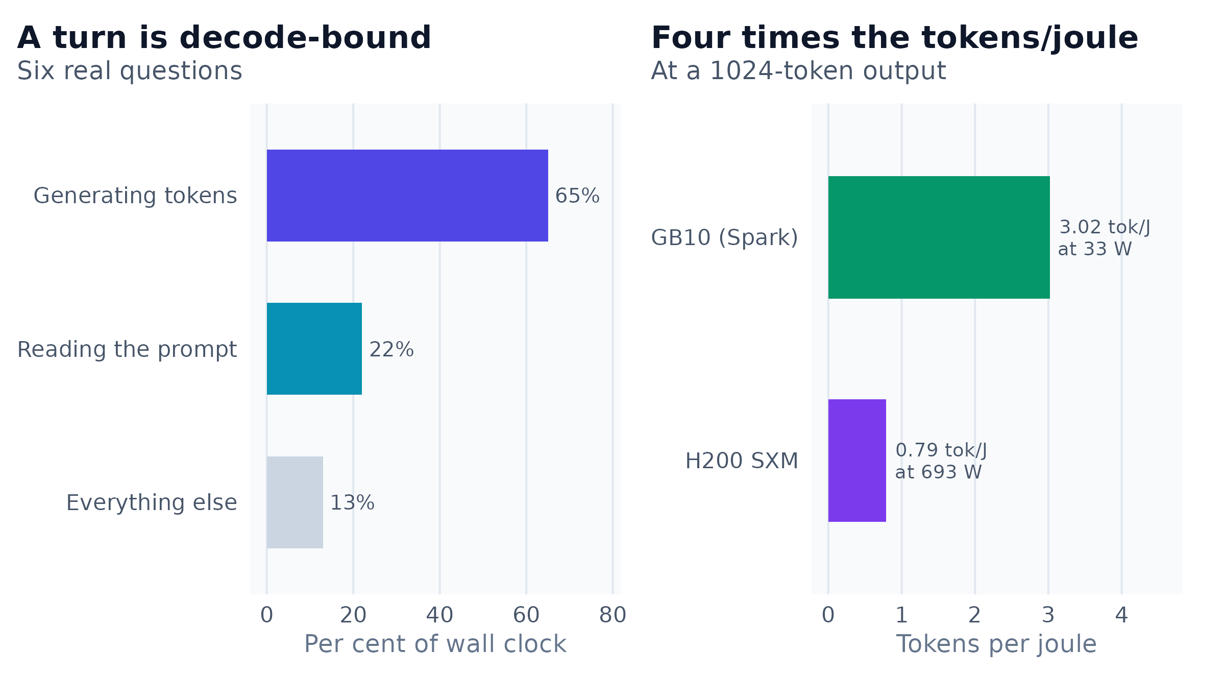
Figure 10: Composition of a median assistant turn, and generation energy for the two machines. The turn is decode-bound, which is why speculative decoding is the lever that matters and additional prefill throughput would buy about a fifth of it.
The energy comparison requires a caveat. The Spark’s thirty-three watts is the whole module, processor and memory included, while the H200’s 693 watts is the accelerator board alone and excludes its host. The true system-level gap is therefore wider than four times, not narrower. Either way, a twenty-one-fold difference in power for a 2.6-fold difference in throughput is the entire argument for putting a model on a desk.
The machine also does not derate under sustained load. Over seventy-eight consecutive load windows, throughput fell 1.5 per cent, peak temperature reached 81 degrees, power averaged 88 watts, and no throttling was reported.
Part II: Training a language model
The training comparison reuses a pretraining run already under way on the cluster: a 2.06-billion-parameter decoder being trained from scratch, whose production configuration occupies three H100s and was 26.5 billion tokens into a 110-billion-token schedule at 9.02 seconds per step when these measurements were taken.
Everything below holds constant the model code, the recipe, the optimizer, the sequence length, the gradient checkpointing policy and the data, and varies only the card. The parameter count was verified identical on both architectures at 2,063,667,712. Two things cannot be held constant and are disclosed rather than corrected: the Spark requires CUDA 13 and therefore a newer PyTorch than the cluster’s driver permits, and the Spark’s power figure covers the whole module while the datacenter cards’ covers the board.
Throughput
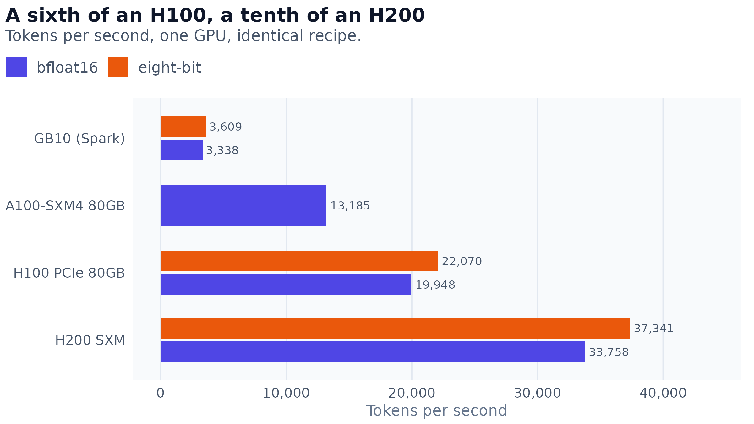
Figure 11: Training throughput for an identical 2.06-billion-parameter recipe on one GPU, at each card’s best configuration. Missing bars are not omissions: an L40S with 48 GB cannot hold this recipe at any batch size, and eight-bit training is unavailable before the Hopper generation.
Two observations that a single ratio hides. The forty-eight-gigabyte L40S fails at every batch size tried, because thirty-two-bit master weights plus the optimizer’s two moment estimates for 2.06 billion parameters occupy about thirty-three gigabytes before a single activation is stored. The Spark’s 121.7 GiB holds the recipe comfortably. And eight-bit training does not merely underperform on an A100, it does not run: the arithmetic format the recipe requires was introduced with the Hopper generation, and the compiler reports the type as unsupported.
Tuning is worth more than three times
The first measurement taken on the Spark was 1,149.9 tokens per second. The last was 3,608.6, on the same hardware and the same model.
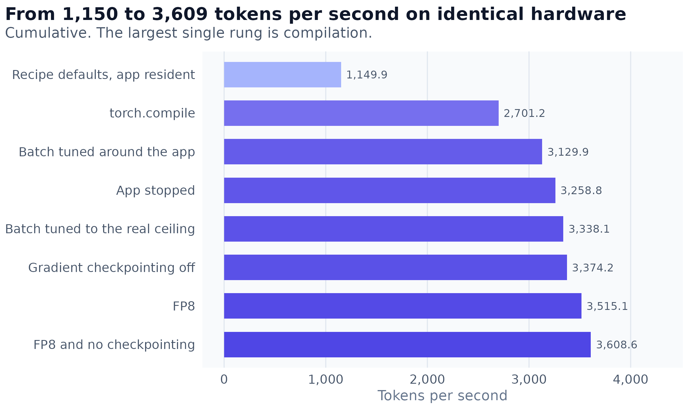
Figure 12: Each successive change to the training configuration on the Spark, cumulative. The largest single contribution is compilation. The fourth rung is not a software change: it is stopping the inference engine that shares the memory pool.
Compilation alone is worth 2.35 times, and the same multiplier appears on the H100, so it is not an artefact of the unusual architecture. Two rungs are worth dwelling on.
Eight-bit precision is the best single knob on this machine, and not primarily for speed. It gives 3,608.6 tokens per second against 3,338.1 for the best sixteen-bit configuration, using sixteen fewer gigabytes at twenty-two per cent less power. In energy terms that is 60.6 tokens per joule against 41.7, an improvement of forty-five per cent. On a machine whose case for existing is energy, that is the number that matters.
Gradient checkpointing turns out not to matter. The recipe enables it by default, which is correct on an eighty-gigabyte card where activation memory binds. Disabling it on the Spark is worth thirteen per cent at a fixed batch size. But checkpointing frees memory, that memory converts into batch size, and at each policy’s own best batch the two are 1.1 per cent apart. The honest advice is that either is fine and this is not where the wins are, which is duller than the fixed-batch comparison suggests and is what a practitioner should act on.
The optimal sequence length belongs to the model, not the card
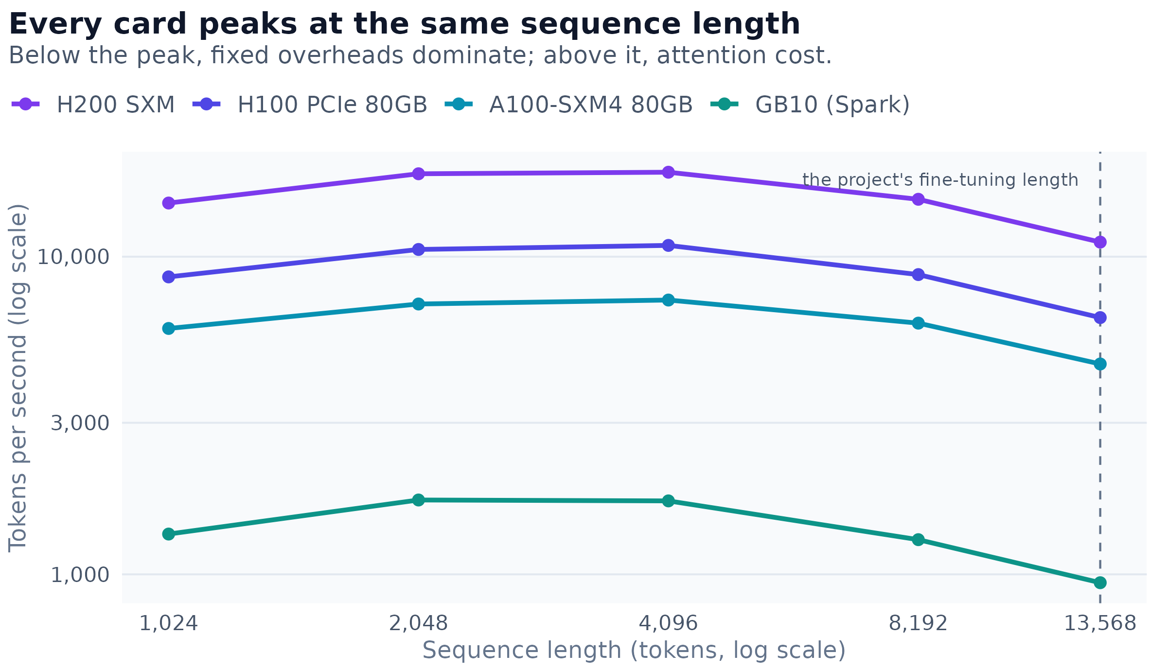
Figure 13: Training throughput against sequence length at a fixed micro-batch of one, on four cards spanning an eightfold range of arithmetic throughput. Every card peaks between two and four thousand tokens. The vertical marker is the sequence length the project’s own fine-tuning configuration uses.
The peak sits between two and four thousand tokens on every card, across a 7.9-fold range of arithmetic throughput and a 14-fold range of bandwidth. It is therefore a property of the model’s shape rather than of the hardware, which makes it a portable tuning result: choose the sequence length once for the model. Beyond the peak, a fine-tune at 13,568 tokens pays roughly 1.7 times per token what the same model pays at 4,096, on every card, within two per cent.
Does the Spark train the same model?
Every figure so far measures how fast the Spark trains. None of them would notice if its arithmetic diverged, and there is reason to think it might: a different PyTorch on a different processor architecture selects different attention and reduction kernels, so bit-identical results are impossible. If the loss trajectory drifted, the claim that one can pretrain on this machine would be wrong for a reason no throughput benchmark could detect.
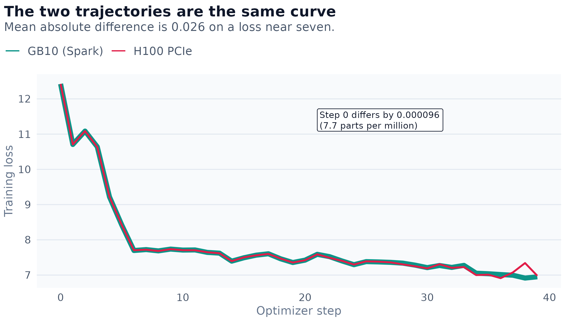
Figure 14: Training loss over forty optimizer steps from a fresh initialisation on each card, with identical seed, recipe, optimizer and tokens at identical offsets, compilation disabled and sixteen-bit arithmetic on both sides. The inset value is the difference at the first step, before any accumulated divergence is possible.
The first step agrees to 7.7 parts per million, which is the important result: the weight initialisation, the data pipeline and the forward pass are equivalent across the two software stacks. From there the runs drift as two valid but different floating-point kernel selections should, by 0.37 per cent on average, with total loss reduction matching within 0.6 per cent. The trajectories stay parallel. The Spark trains the same model, roughly six times more slowly.
This comparison very nearly produced a wrong answer. The first attempt had the two cards reading differently sized data files, and because the batch sampler draws offsets from the file length, the two runs saw entirely different tokens. The resulting trajectories differed by a plausible-looking 1.88 per cent, which measured the data rather than the arithmetic. Pinning the addressable range to an identical size on both sides is what produced the figure above.
The capability no single datacenter card has
The most interesting training result on this machine is not a rate. Consider fine-tuning the thirty-billion-parameter model with low-rank adaptation, which trains a small number of added parameters while the base model stays frozen.
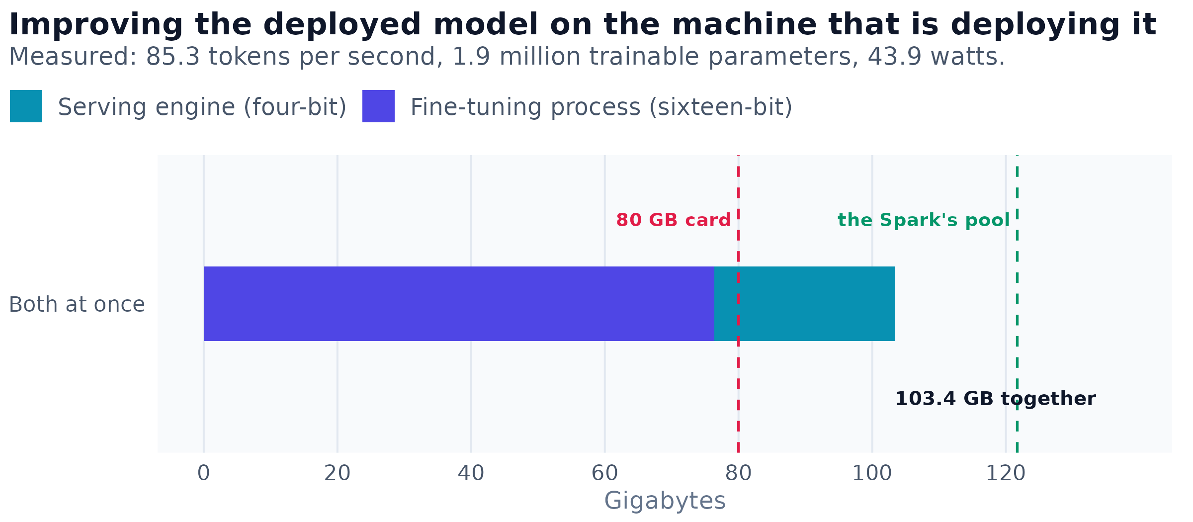
Figure 15: Memory required to fine-tune the thirty-billion-parameter model with low-rank adaptation while simultaneously serving it, against what two accelerators provide. Both components are measured: 76.4 GB for the fine-tuning process and 27 GB for the serving engine. The dashed line is an eighty-gigabyte card’s capacity.
Low-rank adaptation of this model runs at 85.3 tokens per second in 76.4 gigabytes, training 1.9 million parameters, or 0.0059 per cent of the model, at 43.9 watts. Add the twenty-seven gigabytes the serving engine was measured holding and the pair needs 103.4 gigabytes of the available 121.7. An eighty-gigabyte card can host the fine-tuning run or the served copy, but not both.
At 85.3 tokens per second that is about 307,000 tokens an hour, or 7.4 million a day: a few-million-token adaptation pass is an overnight job on a machine that is otherwise idle overnight. It is not a machine for a ten-billion-token fine-tune. But the shape of the work it enables, improving a deployed model on the hardware that deploys it, with no second machine and no maintenance window, is genuinely unavailable on a single datacenter accelerator.
Part III: Serving a model larger than the machine
The measurements so far hold the model fixed and ask how fast the machine runs it. This part asks the opposite question. A mixture-of-experts model routes each token through a small subset of its expert feed-forward networks, so the parameter count grows without the per-token arithmetic growing with it. That makes weight movement, rather than arithmetic, the binding constraint, and it opens a possibility that a dense model does not have: the experts can live in host memory and be fetched as they are needed, so the model no longer has to fit in accelerator memory at all.
What FreeToken is
FreeToken is an open-source mixture-of-experts serving engine from FlashML, released under the Apache 2.0 licence and described in FreeToken: Efficient Edge-Native MoE Serving with Bandwidth-Adaptive Execution, a paper by Yang and ten co-authors posted four days before this article. Its premise is the one above, and the paper’s framing of that premise is worth borrowing because it is also this article’s: treat a personal machine “not as a small GPU, but as a unified, elastic inference platform”. The claim attached to it is a large one. The paper reports serving a 35-billion-parameter model on a laptop GPU and a 753-billion-parameter model on a workstation card, and the project’s own summary offers frontier models on a gaming PC. What follows takes that claim seriously enough to measure it.
The mechanism doing the work is a cache. Expert weights sit in host memory, a fixed number of slots in accelerator memory hold the most recently used of them, and a token routed to an expert that is not resident waits for that expert to cross the interconnect. Around this sit further pieces the paper names and these measurements do not separate out: a bandwidth-adaptive policy for deciding how much of an expert’s arithmetic to run on the CPU rather than move its weights to the GPU, prefill that fetches one layer’s experts while the previous layer computes, and the ability to shift accelerator memory between the expert cache and the key-value cache without restarting the engine. The cache is what the rest of this part measures, because it is the part that decides whether an oversized model runs at a usable rate or does not run at all.
The engine is a closer relative of Part I’s software than it first appears. Its acknowledgments credit design and reused code to SGLang, vLLM, FlashInfer, LightLLM and llama.cpp, so what is being compared here are relatives rather than strangers. It is also early software. The version measured is 0.1.2, which its own packaging marks as beta, and whose registry names twenty-four model architectures across fourteen families. Not everything measured below is a property of the machine: one result is a defect in a single engine code path, and another is an allocation choice that costs nothing except on unified memory. The text says which.
FreeToken is also the first piece of software in this article that the Spark is qualified to run and the datacenter cards are not: it requires a CUDA 13 driver, which the Spark has at 580.159.03 and the A100 nodes do not, their driver topping out at CUDA 12.2. Running it on the A100 for comparison required installing it against the older toolkit and rebuilding the two extensions it ships, which are linked against a CUDA 13 runtime.
Models that do not fit
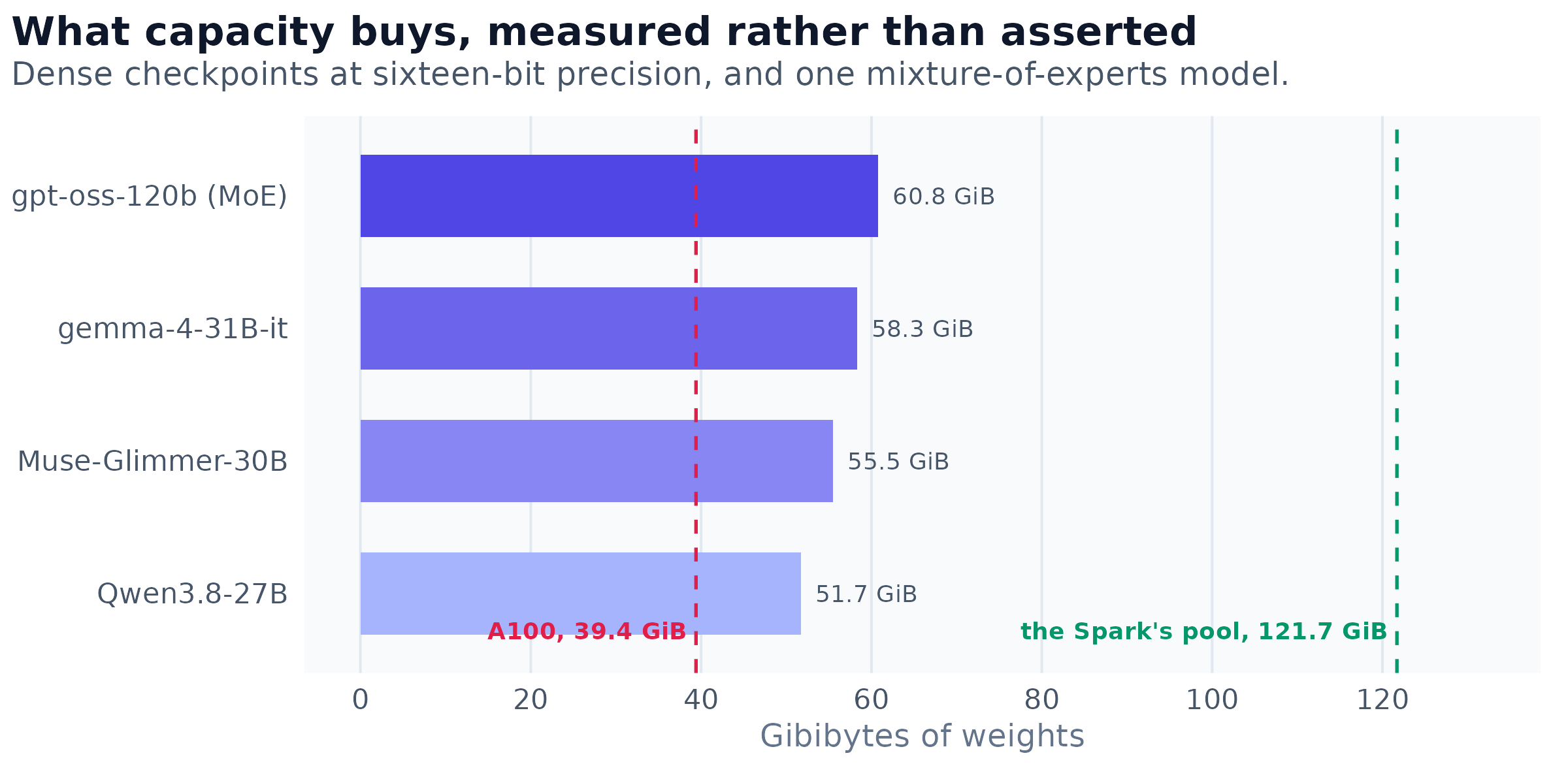
Figure 16: Weights of four checkpoints against the two machines’ capacities. The three dense models between 51 and 59 gigabytes exceed a 40 GiB card and were measured failing on it, short by 170, 254 and 222 mebibytes respectively; all three load and answer correctly on the Spark. The mixture-of-experts model at the bottom exceeds the card as well, but its experts can be held in host memory, which is the subject of the next figure.
Part IV argues that the capacity is for models too large for a datacenter card. These are those models. The three dense checkpoints do not fail marginally on the A100 and they do not fail for want of tuning: the card runs out of memory with the weights nearly resident and nothing left for the key-value cache. On the Spark all three answer correctly, at three to four tokens per second, which is a rate for batch work rather than conversation.
What it costs to keep the experts in host memory
A mixture-of-experts model can go further, because only the experts a token actually routes to are needed for that token. FreeToken keeps them in host memory and maintains a cache of expert slots in accelerator memory, streaming the misses across the link. The size of that cache is the one setting that matters.
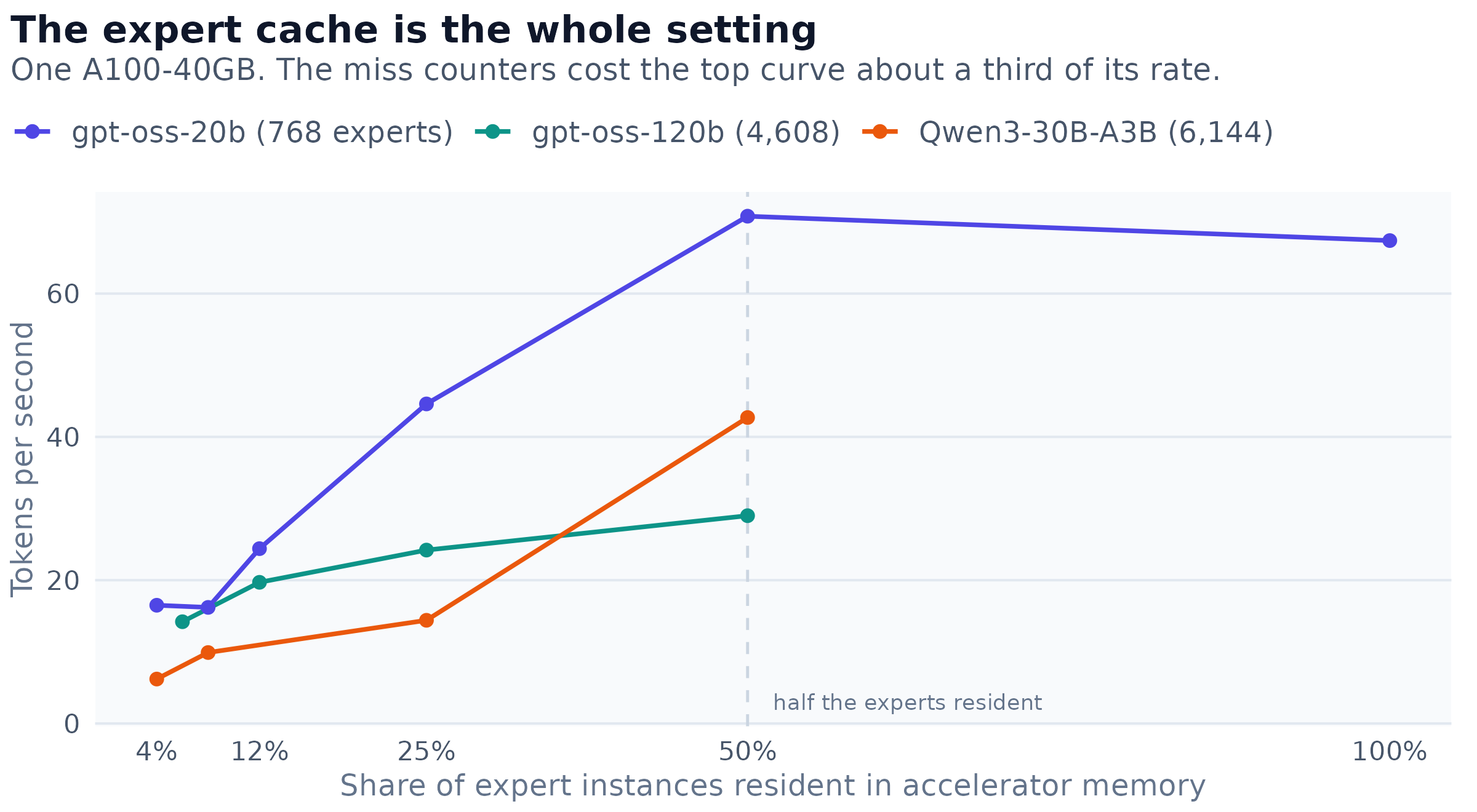
Figure 17: Decode rate against the fraction of expert instances held in accelerator memory, for three mixture-of-experts models on one A100. The vertical marker is fifty per cent residency, where the realised miss rate was 9.0 per cent for gpt-oss-20b, 6.4 for gpt-oss-120b and 4.0 for Qwen3-30B-A3B. Below a quarter the rate falls steeply; above a half there is nothing left to buy. The two larger models cannot hold all of their experts at any setting, which is why their curves stop short of the right edge.
Two properties of these curves are worth more than the rates themselves. The first is that half is enough: at fifty per cent residency the realised miss rate stayed below ten per cent for all three models, because consecutive tokens reuse experts heavily. The second is that the floor is set by the link and can be predicted without running anything. For gpt-oss-20b, each expert is 12.61 mebibytes of four-bit weights, a token routes to four of them in each of twenty-four layers, and 1.182 gibibytes at the measured 21.5 GiB/s of pinned host-to-device bandwidth gives 18.2 tokens per second. The measured floor is 16.2, or 89 per cent of that bound, which is as close as a bandwidth argument usually gets.
The Spark changes this arithmetic rather than the mechanism. Its host-to-device path measured 55.19 GiB/s against the A100’s 21.5, because there is no bus to cross, and holding experts in “host” memory there means holding them in the same physical memory the GPU is already using. The engine’s own calibration reports the same asymmetry from the other side, at 81.0 against 25.2 gigabytes per second.
On the Spark that arithmetic has a second term, and it is the one that decides the outcome. Asking for offloaded experts there allocates them twice: once as the pinned host-side bank and once as the resident slot cache the engine gathers into. On a discrete card those are two different memories. Here they are one, so requesting offload for a model that already fits costs twice the model’s memory to hold the same weights.
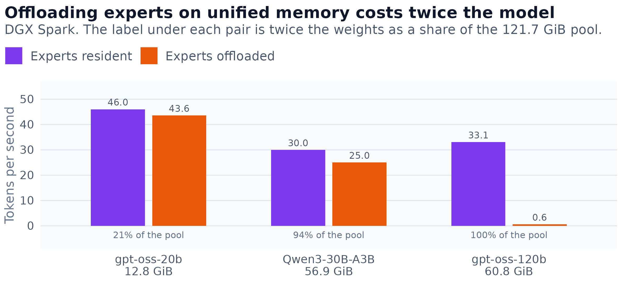
Figure 18: Decode rate on the Spark for the resident-expert backend and the offloading one, against twice the weights as a share of the machine’s pool. Offload holds the experts as both a host-side bank and a resident cache, so the memory it needs is twice the model. At a fifth of the pool that costs nothing; at ninety-four per cent it costs seventeen per cent; at the pool’s capacity the machine was left 1.19 GiB free and the rate fell to 0.6 tokens per second.
I had taken the first two of these measurements to mean that the cost of offloading tracks the number of experts, which was 768 and then 6,144. The third refutes it: gpt-oss-120b has fewer expert instances than Qwen3-30B-A3B and four gibibytes more weights, and it is the one that collapses. What the cost tracks is how close twice the model comes to the pool. The guidance is therefore simple and specific to this machine: offload experts only when the model does not otherwise fit, and never as a default.
Concurrency does not rescue a cache that is too small
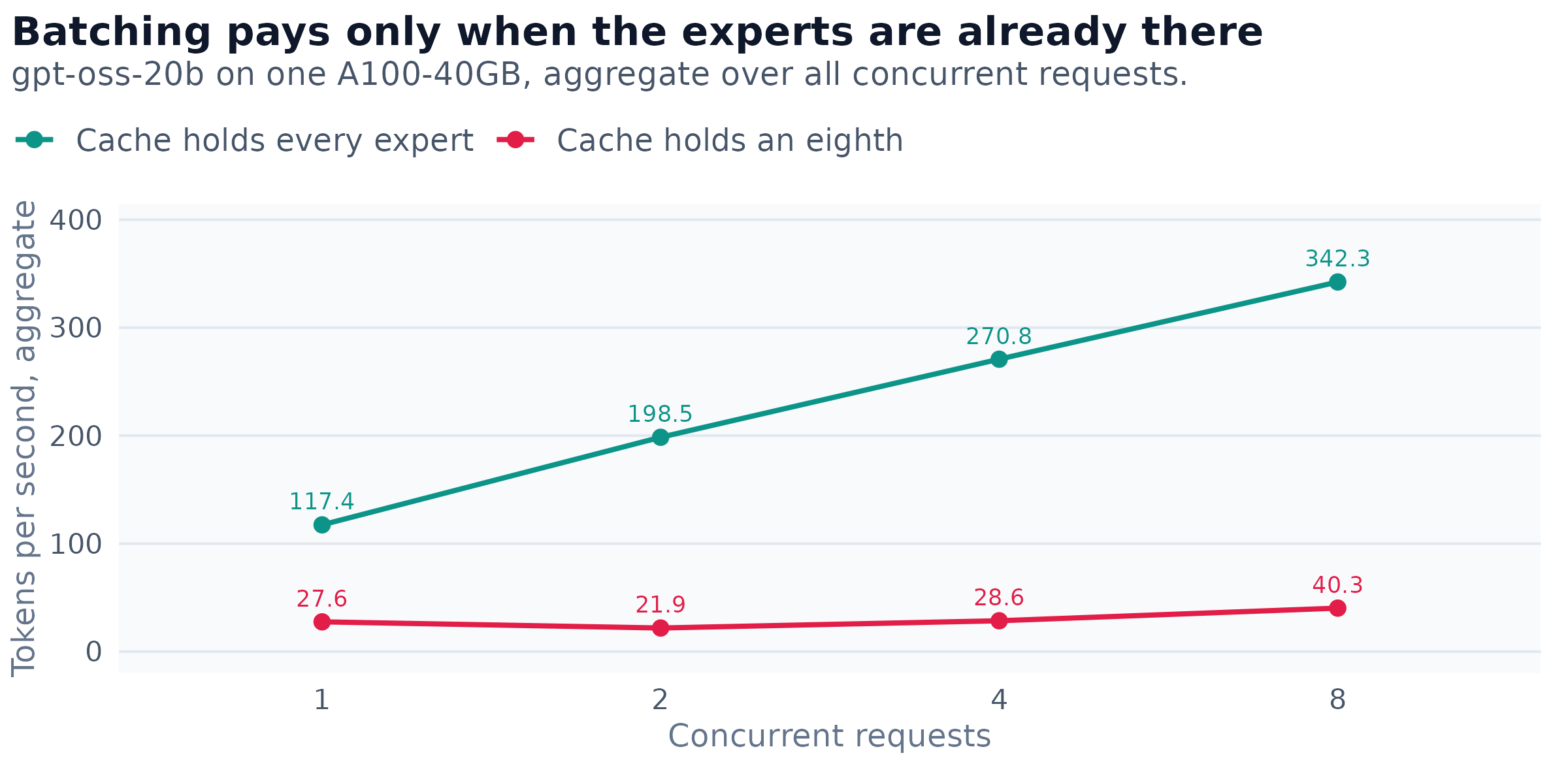
Figure 19: Aggregate throughput against the number of concurrent requests, for the same model and engine on one A100, with the expert cache sized to hold every expert and sized to hold an eighth of them. When the cache fits, eight concurrent requests return 2.9 times the throughput of one. When it does not, they return 1.5 times, because the number of distinct experts a single step needs grows with the batch, from 4.0 per layer at one request to 13.9 at eight.
This is the operational rule that follows from the mechanism. Batching amortises a fetched expert over several tokens only if the fetch is shared, and a larger batch routes to more distinct experts, so an undersized cache thrashes harder as concurrency rises. Size the cache first, then batch.
Four-bit weights, and which four-bit weights
The serving results in Part I already show that quantisation is worth more to this machine than to one with bandwidth to spare. The same holds for models too large to serve otherwise, and with a larger effect on what fits.
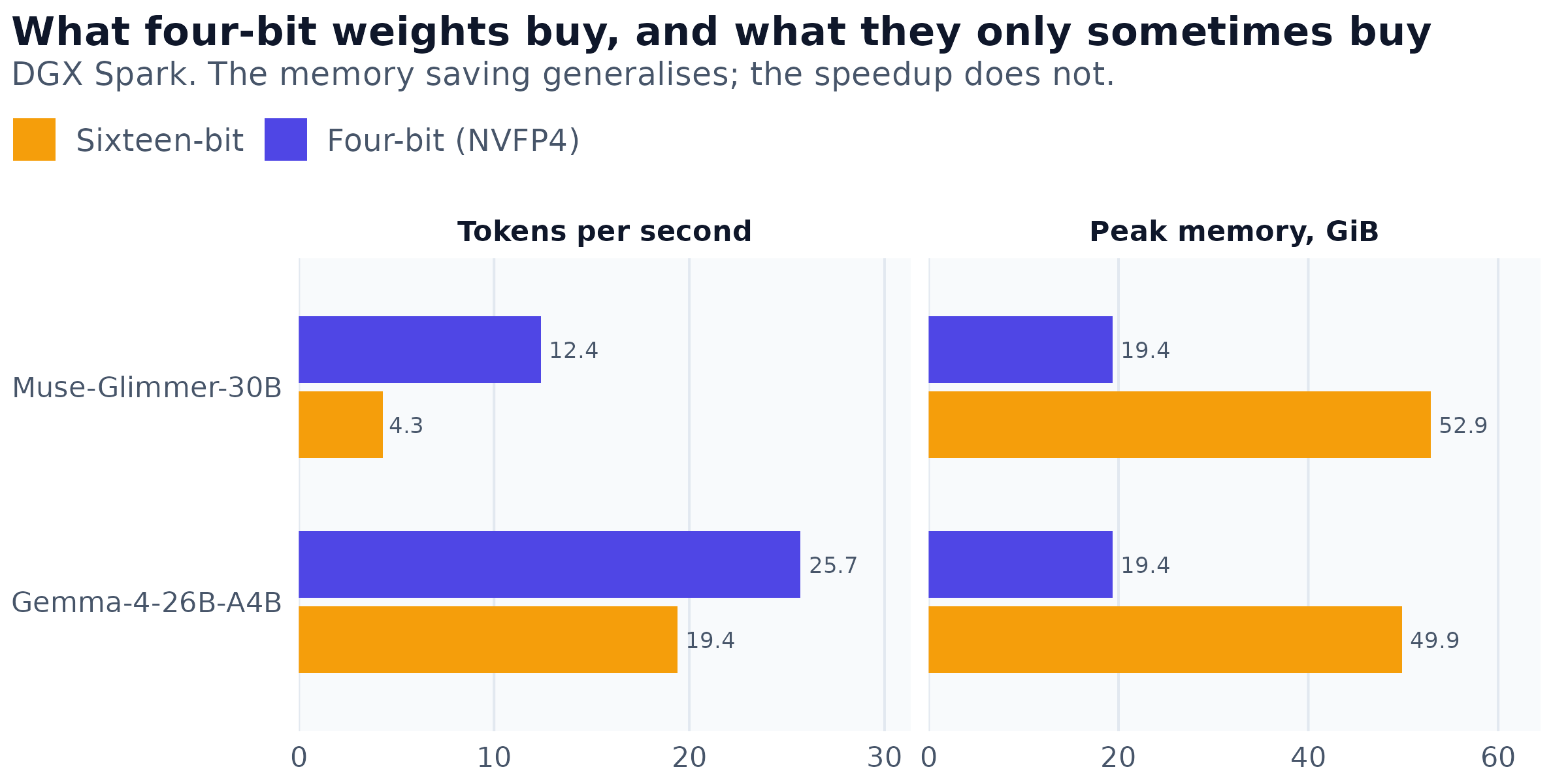
Figure 20: Two models on the Spark at sixteen-bit and four-bit precision. Four-bit weights reduce peak memory by a factor of 2.6 to 2.7 in both cases, which is the reliable part. The decode gain is not reliable: it is 2.9 times for one model and 1.32 times for the other, and prefill did not move for the second at all.
The memory saving is the dependable half and it is the half that decides what runs at all. The speed gain varies by more than a factor of two between two models in the same format on the same machine, so it should be measured per checkpoint rather than assumed.
A sharper version of that caution appeared on the A100, where two checkpoints in nominally the same four-bit format differed by a factor of twenty.
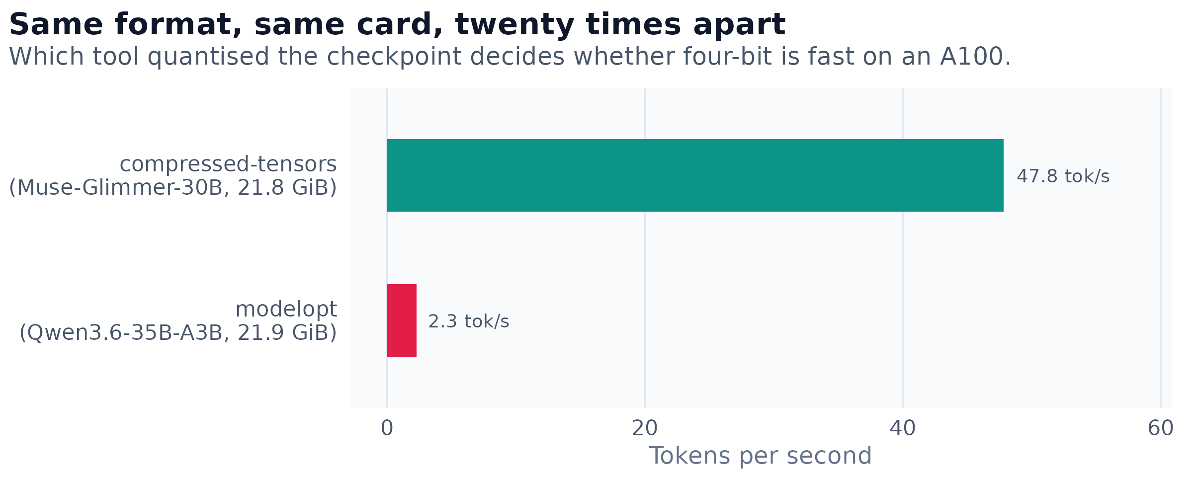
Figure 21: Decode rate on one A100 for two four-bit checkpoints of comparable size, both nominally NVFP4. The only relevant difference is which tool produced them, recorded in the checkpoint as quantization_config.quant_method. The slower path also refuses the resident-expert backend, which the faster one accepts.
I had concluded from the first of these two checkpoints that four-bit weights were a severe pessimisation on an A100, and that four-bit inverted which of the two machines was faster. The second checkpoint refuted both statements. What the format is called does not determine how it performs; the implementation behind the name does, and the field that identifies it is in the checkpoint’s own configuration.
A limit worth stating
Two of the largest models tried did not produce a serving result, and the reasons are different. DeepSeek-V4-Flash, at 155.4 gibibytes with 11,008 expert instances, staged completely onto one A100: sparse attention selected, key-value pages resized to its requirement, expert banks built in host memory, four gigabytes of accelerator memory still free. Generation then failed during CUDA graph capture in every configuration attempted, including the smallest legal expert cache, so it was not a shortage of working memory. Making kernel launches synchronous located the cause in the sparse-attention indexer, which launches with a grid computed from a value only known at run time; a launch shape that varies inside a capture region invalidates the graph. That is a defect in one code path rather than a limit of the machine.
The other limit is the machine. This model cannot run on the Spark at all, because 155.4 gibibytes do not fit a 121.7 gibibyte pool, and the manoeuvre that makes an oversized model possible elsewhere is unavailable here: holding experts in host memory adds no capacity when host memory and accelerator memory are the same memory. The A100 node, with a smaller accelerator and 250 gigabytes of separate host memory, hosts a strictly larger mixture-of-experts model than the Spark does. That is the sharpest statement of the trade in this article: unified memory is what lets one modest machine hold a large model and a training run at once, and it is also what stops it holding a model larger than itself.
Part IV: What the machine is for
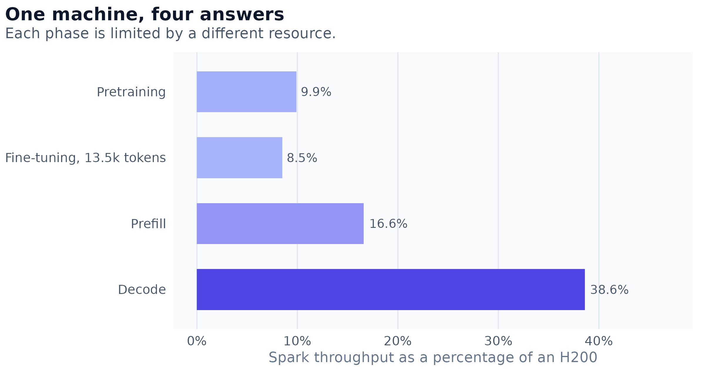
Figure 22: The Spark’s throughput as a percentage of each datacenter card’s, by phase of work. Training and fine-tuning were measured on all three cards. Prefill and generation were measured against an H200 only, which is the fastest of the three, so those two bars understate the Spark relative to an H100 or an A100 rather than flattering it.
This is the article’s central result. Against an H200 the Spark is a tenth at training, a sixth at reading prompts, and two fifths at generating tokens; against an A100 it is a quarter at training. The spread within a single machine is wider than the spread between the cards it is being compared with, because those activities are limited by different things. Generation is the phase where quantisation works hardest, and quantisation is worth far more to a bandwidth-starved machine than to one with bandwidth to spare. The same four-bit weights that buy the Spark nothing on a training step buy it most of its serving performance.
The two serving rows carry a caveat the training rows do not: the serving suite was run against one datacenter card, an H200. Since that is the fastest of the three measured for training, those two percentages are the least favourable comparison available rather than the most, and the corresponding figures against an H100 or an A100 would be higher.
That asymmetry is the design guidance. Put interactive serving of a quantised model on this hardware, where it performs within a factor of two or three of a datacenter card at a twentieth of the power. Put throughput training on the datacenter cards, where the gap is a factor of ten. Use the memory capacity for the things capacity buys: models too large for eighty gigabytes, and combinations of workloads that will not otherwise coexist.
The cost of sharing one pool
Everything on this machine competes for the same 121.7 GiB, and that has a price. A co-resident job costs the serving application seventy-four to seventy-seven per cent of its generation rate, measured twice by different means. In the other direction, the serving engine’s twenty-seven gigabytes cost a training run six per cent of its peak throughput once the batch size is re-tuned around it, and twenty-four per cent if it is not.
That last distinction was expensive to learn. An earlier version of these measurements concluded that filling memory on this machine was actively counterproductive, because throughput collapsed twenty per cent as the batch grew. Repeating the identical configurations with the serving engine stopped, the same batches recovered completely and the largest became the fastest. The collapse was contention with a neighbour, not a property of unified memory, and only running both conditions revealed which.
Two failure modes that do not exist on a discrete card
Unified memory removes the boundary between host and accelerator, and with it two guarantees that ordinary GPU code relies on.
A configuration that would merely fail on a discrete card can stop the whole machine. Requesting an over-large batch on an H100 raises an out-of-memory error, the harness catches it, prints a line, and continues; this happened repeatedly during these measurements and cost nothing. The same request on the Spark draws from the pool the operating system is using. A fine-tuning configuration needing about 151 gigabytes of a 121.7-gigabyte machine did not fail: it took the host off the network for two and a half hours, and the kernel eventually resolved it by killing the serving engine. The machine has sixteen gigabytes of swap, which is precisely what converts an immediate clean failure into a prolonged one. The diagnostic that distinguishes a healthy memory-heavy run from a dying one is the kernel’s own pressure metric rather than free memory: a later run holding eighty-seven gigabytes reported zero stall at ninety-six per cent utilisation, while the incident ran at a load average of fifty-eight.
Capacity planning must count the page cache. A second attempt to fine-tune the thirty-billion-parameter model was killed seventy-three per cent of the way through loading its weights, with room to spare on paper: fifty-seven gigabytes of weights plus a twenty-seven-gigabyte engine is eighty-four of 121.7. What the arithmetic omitted was eighty-two gigabytes of page cache, left over from having written the sixty-two-gigabyte checkpoint to disk minutes earlier. Because those file pages were actively mapped rather than clean and evictable, the kernel killed the loader instead of reclaiming them. On a discrete card the page cache lives in host memory and is irrelevant to what fits in accelerator memory. Here they are the same pool, and a recently touched file is occupied memory.
A related trap sits in the most ordinary line of model-loading code. Reading a checkpoint to host memory and then copying it to the device is two allocations of different memory on a discrete card, and two allocations of the same memory here: a fifty-seven-gigabyte model transiently needs 114 gigabytes. Pinning each shard directly to the device as it is read keeps the peak at one copy.
The serving work in Part III met the same accounting from the other direction, which is worth recording because the symptom was not an out-of-memory error. FreeToken sizes its key-value cache from the free memory the driver reports once the weights are resident, and on this machine that figure is the kernel’s count of free pages, which the checkpoint’s own read has just consumed. Loading a 51.7-gigabyte model with 114.9 gibibytes free beforehand left the solver deciding it had room for less than one page, and it refused to start. Advising the kernel to drop those specific file pages, with posix_fadvise over the checkpoint, returned free memory from 61 to 115 gibibytes and needed neither administrative rights nor a large allocation to force reclamation.
None of these are arguments against the machine. They are the cost of the property that makes it interesting, and all three are avoidable once known.
Notes on method
Every number here comes from a harness that ran on the hardware described, and the underlying result files are retained alongside the analysis. Three practices did more than the rest to keep the conclusions honest, and are worth stating because in each case the alternative had already produced a wrong answer.
First, the harness reports what it actually did, and that report gets read. An eight-bit training comparison recorded a suspiciously exact absence of any effect, and the effect was absent because the quantisation library was not installed: the harness had recorded the failure faithfully in its output and the field had not been examined. Reinstalled, the same configuration gives ten per cent.
Second, when a comparison yields a small and plausible difference, the first thing to check is that both sides varied only in the intended dimension. This caught the numerics comparison described above, and it caught the eight-bit one.
Third, a claim measured once is a claim measured under one set of conditions. Two of this article’s more quotable early findings, that filling memory is counterproductive and that eight-bit precision does nothing here, were artefacts of the environment rather than properties of the hardware, and both survived until something forced a re-measurement.
Conclusion
A desktop machine with one small GPU and a large shared memory pool is not a substitute for a datacenter accelerator, and it is not trying to be. It trains a two-billion-parameter model at a sixth of an H100’s rate, and it trains the same model: the loss curves agree to seven parts per million at the first step and remain within a percentage point of each other.
What it is instead is a machine with a different balance of resources, and the balance favours exactly the workload described in the first half of this article. Serving a quantised model to a handful of interactive users, it reaches two fifths of an H200’s generation rate at a twentieth of the power, holds that rate out to fifty-eight thousand tokens of context, answers with no measurable loss of quality relative to sixteen-bit precision, and never throttles. It will additionally hold a fine-tuning run for the same model alongside the copy it is serving, which no single eighty-gigabyte card will do.
The assistant behind these numbers has been answering questions about a supercomputing centre, from a corpus that never leaves the building, on a computer that fits under a desk and draws less power than a bright light bulb.