Ramen Ratings LASSO Prediction & Visualization

LASSO Model: Using variety words to predict ramen rating

variety_matrix <- ramen_ratings  %>%
  mutate(row_id = row_number()) %>%
  unnest_tokens(word, variety) %>%
  anti_join(stop_words) %>%
  distinct(row_id, word) %>%
  add_count(word) %>%
  filter(n > 10) %>%
  cast_sparse(row_id, word) 
  

# Lining up stars with row_id

row_id <- as.integer(rownames(variety_matrix)) 

stars <- ramen_ratings$stars[row_id]

cv_glmnet_model <- cv.glmnet(variety_matrix, stars)

plot(cv_glmnet_model)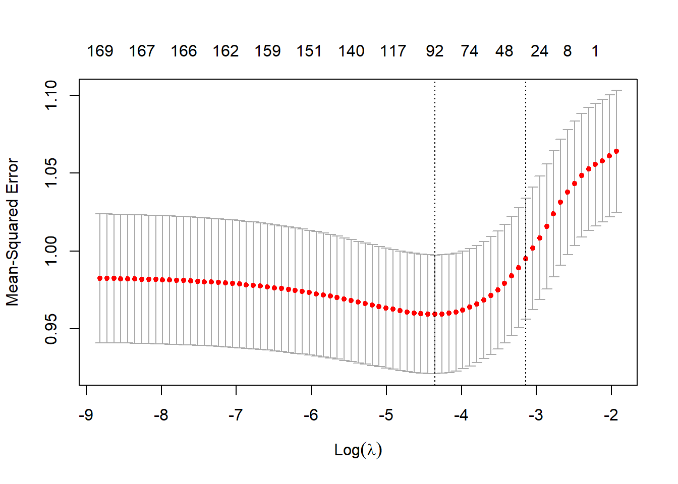

cv_glmnet_model$glmnet.fit %>%
  tidy() %>%
  filter(!str_detect(term, "(Intercept)"),
         lambda == cv_glmnet_model$lambda.1se) %>% 
  select(word = term, coefficient = estimate) %>%
  mutate(direction = if_else(coefficient < 0, "negative", "positive")) %>%
  group_by(direction) %>%
  slice_max(abs(coefficient), n = 20) %>%
  ungroup() %>%
  mutate(word = fct_reorder(word, coefficient)) %>%
  ggplot(aes(coefficient, word, fill = word)) +
  geom_col(show.legend = F) +
  labs(x = "estimated coefficient",
       y = "word",
       title = "How does the description word impact ramen rating?")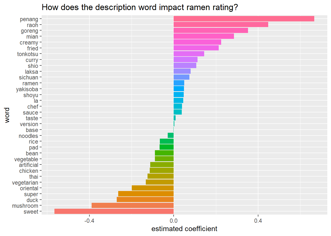

Ramen Style & Country on Rating

ramen_majority <- ramen_ratings %>%
    filter(style %in% c("Bowl", "Cup", "Pack", "Tray"))

ramen_majority %>%
  mutate(country = fct_lump(country, n = 10)) %>%
  ggplot(aes(stars, country, fill = country)) +
  geom_violin(show.legend = F) +
  facet_wrap(~style, scales = "free_y") +
  labs(y = NULL,
       x = "rating",
       title = "Ramen Rating for Top 10 Countries Faceted by Style",
       subtitle = "Top country is defined by the # of ramen it has") +
  theme(strip.text = element_text(size = 15, face = "bold"),
        axis.title = element_text(size = 14),
        axis.text = element_text(size = 13),
        plot.title = element_text(size = 18),
        plot.subtitle = element_text(size = 14)
        )

## Warning: Groups with fewer than two data points have been dropped.

## Warning: Groups with fewer than two data points have been dropped.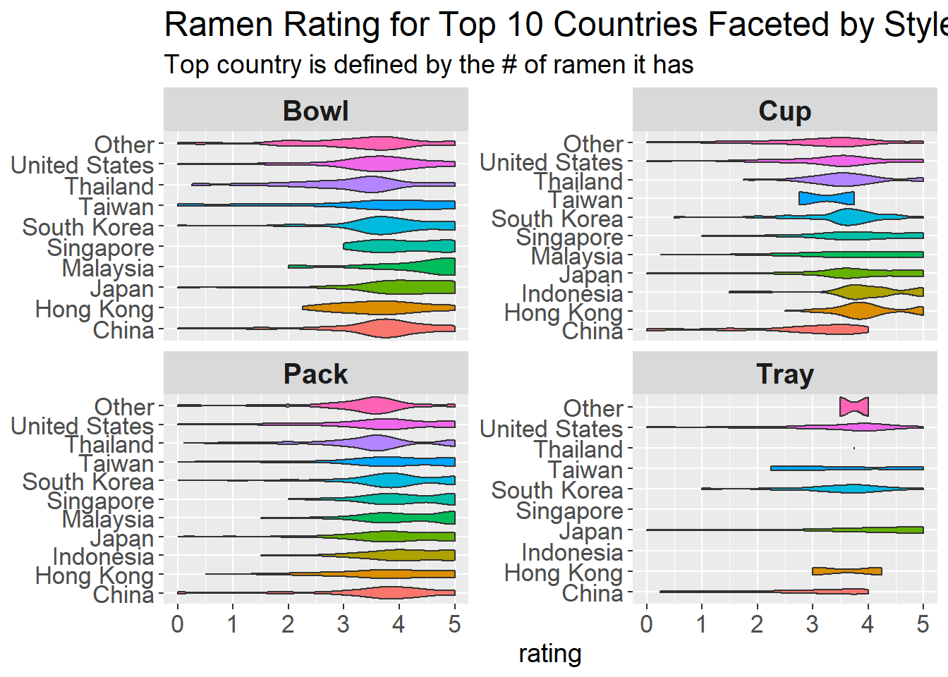

International ramen brands

international_brands <- ramen_majority %>%
  count(brand, country, sort = T) %>%
  count(brand, sort = T) %>%
  filter(n > 1) %>%
  pull(brand)

ramen_international <- ramen_ratings %>%
  filter(brand %in% international_brands)

International brand count in each country

ramen_international %>%
  filter(style != "Box") %>%
  count(brand, style, country, sort = T) %>%
  mutate(brand = reorder_within(brand, n, style, sum)) %>%
  ggplot(aes(n, brand, fill = country)) +
  geom_col() +
  facet_wrap(~style, scales = "free_y") +
  scale_y_reordered() +
  labs(y = NULL,
       x = "count",
       title = "International Ramen Brand Count Per Country Faceted by Style") +
  theme(strip.text = element_text(size = 15, face = "bold"),
        axis.title = element_text(size = 14),
        axis.text = element_text(size = 9),
        plot.title = element_text(size = 18),
        legend.title = element_text(size = 9),
        legend.text = element_text(size = 8)
        )

International brand rating

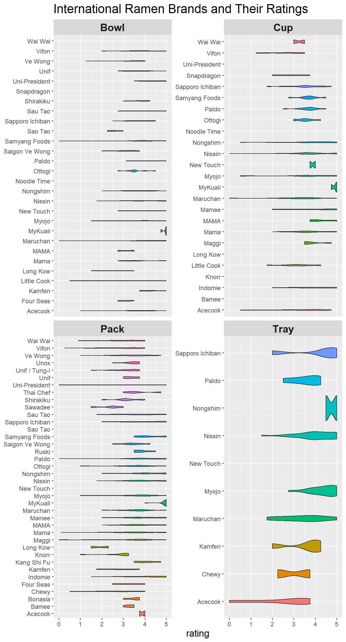
ramen_international %>%
  filter(style != "Box") %>%
  ggplot(aes(stars, brand, fill = brand)) +
  geom_violin(show.legend = F) +
  facet_wrap(~style, scales = "free_y") +
  labs(y = NULL,
       x = "rating",
       title = "International Ramen Brands and Their Ratings") +
  theme(strip.text = element_text(size = 15, face = "bold"),
        axis.title = element_text(size = 14),
        axis.text = element_text(size = 9),
        plot.title = element_text(size = 18),
        legend.title = element_text(size = 9),
        legend.text = element_text(size = 8)
        )

Learning from David

From here to the end of the blog post, everything is inspired/sparked by David Robinson’s code, which is about web scraping and beyond.

ramen_ratings %>%
  #select(-variety) %>%
  pivot_longer(-c(review_number, stars), names_to = "variable", values_to = "value") %>%
  count(variable, value, sort = T) %>%
  group_by(variable) %>%
  slice_max(n, n = 20) %>%
  ungroup() %>%
  mutate(value = fct_reorder(value, n)) %>%
  ggplot(aes(n, value)) +
  geom_col() +
  facet_wrap(~variable, scales = "free")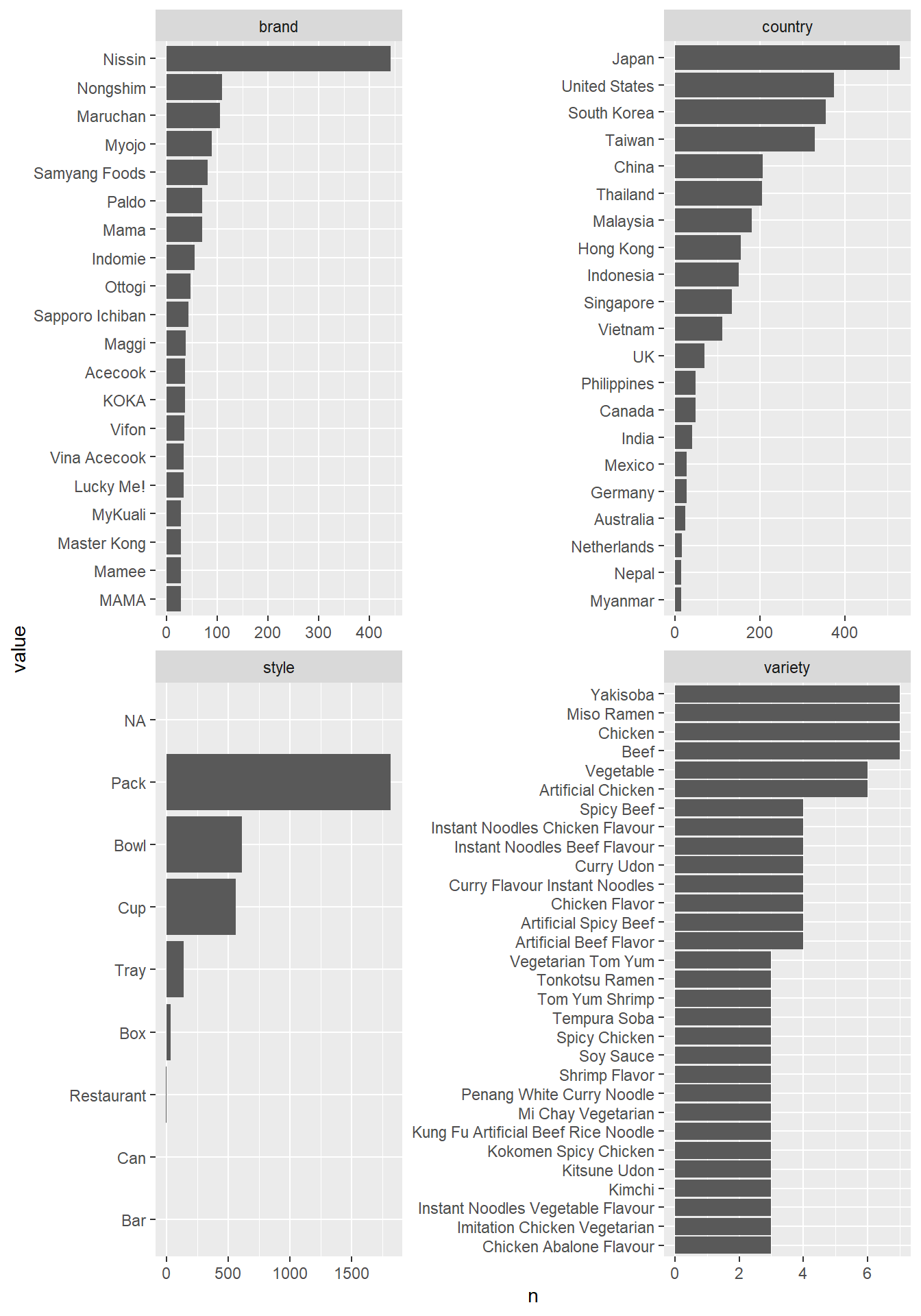

Based on the plot above, we can use fct_lump() to lump some variables.

ramen_processed <- ramen_ratings %>%
  mutate(brand = fct_lump(brand, 20),
         country = fct_lump(country, 10),
         style = fct_lump(style, 4)) %>%
  replace_na(list(style = "Other")) %>%
  mutate(brand = fct_relevel(brand, "Other"),
         country = fct_relevel(country, "Other"),
         style = fct_relevel(style, "Pack"))

Linear model plot

ramen_processed %>%
  lm(stars ~ brand + style + country, data = .) %>%
  tidy(conf.int = T) %>%
  filter(term != "(Intercept)") %>% 
  extract(term, c("category", "term"), "^([a-z]+)([A-Z].*)") %>%
  mutate(term = fct_reorder(term, estimate)) %>%
  ggplot(aes(estimate, term, color = category)) +
  geom_point() +
  geom_vline(aes(xintercept = 0), linetype = 2, color = "orange") +
  geom_errorbarh(aes(xmin = conf.low,
                     xmax = conf.high)) +
  facet_wrap(~category, ncol = 1, scales = "free_y") +
  theme(legend.position = "none") +
  labs(y = NULL)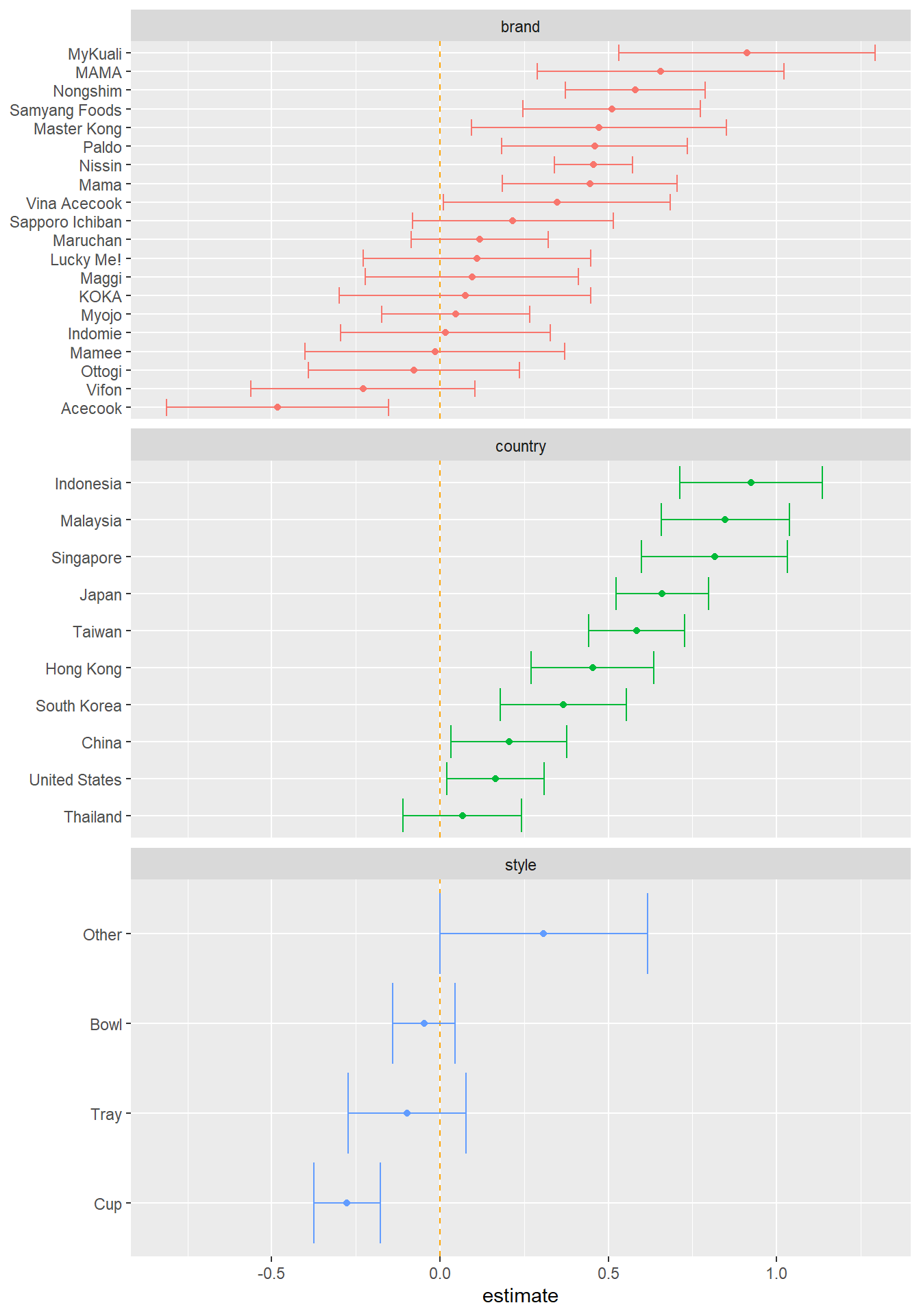

Web scraping

ramen_pages <- tibble(page_num = 1:10)

ramen_pages <- ramen_pages %>%
  mutate(page_link = paste0("https://www.theramenrater.com/page/", page_num, "/"))

get_links <- function(link){
  read_html(link) %>%
    html_nodes(".entry-title a") %>%
    html_attr("href")
}  

ramen_pages <- ramen_pages %>%
  mutate(text_link = map(page_link, get_links))


get_text <- function(link){
  read_html(link) %>%
  html_nodes(".entry-content p") %>%
  html_text() %>%
  as_tibble() %>%
  rename(text = "value") %>%
  filter(text != "")
}

ramen_pages <- ramen_pages %>%
  unnest(text_link) %>%
  mutate(text = map(text_link, get_text)) 

text_df <- ramen_pages %>%
  mutate(text_id = row_number()) %>%
  unnest(text) %>%
  unnest_tokens(word, text) %>%
  anti_join(stop_words) %>%
  filter(!word %in% c("click", "finished", "enlarge", "stars", "detail")) %>%
  distinct(text_id, word, .keep_all = T) 

## Joining, by = "word"

word_cors <- text_df %>%
  add_count(word) %>%
  filter(n > 50) %>%
  filter(str_detect(word, "[a-z]+")) %>%
  pairwise_cor(word, text_id, sort = T) 

word_cors

## # A tibble: 600 x 3
##    item1   item2   correlation
##    <chr>   <chr>         <dbl>
##  1 recipe  cook          0.932
##  2 cook    recipe        0.932
##  3 prepare minutes       0.910
##  4 minutes prepare       0.910
##  5 stir    minutes       0.892
##  6 stir    prepare       0.892
##  7 minutes stir          0.892
##  8 prepare stir          0.892
##  9 finally stir          0.892
## 10 stir    finally       0.892
## # ... with 590 more rows

We can see highly correlated words from word_cors.