Cocktail Visualization & PCA

Working on boston_cocktails

boston_cocktails %>%
  mutate(ingredient = fct_lump(ingredient, n = 10)) %>%
  filter(ingredient != "Other") %>%
  count(category, ingredient, sort = T) %>%
  ggplot(aes(category, ingredient, fill = n)) +
  geom_tile() +
  theme(axis.text.x = element_text(angle = 90),
        panel.grid = element_blank(),
        axis.ticks = element_blank()) +
  scale_fill_gradient2(high = "green",
                       low = "red",
                       mid = "pink",
                       midpoint = 50) +
  scale_x_discrete(expand = c(0,0)) +
  scale_y_discrete(expand = c(0,0)) +
  labs(fill = "ingredient count",
       title = "Top 10 ingredients count among all cocktail categories")

Dealwith with the measure column, which has the complex fractions (e.g. 1 1/2 oz). Tidyevalution is used here to transform the column into a numeric one.

boston_cocktails_oz <- boston_cocktails %>%
  filter(str_detect(measure, " oz")) %>%
  mutate(measure_oz = str_remove(measure, " oz$")) %>%
  mutate(measure_oz = str_replace(measure_oz, "\\s", "+")) %>%
  rowwise() %>%
  mutate(measure_oz = round(eval(parse(text = measure_oz)), 2)) %>%
  ungroup()

Average weight of cocktail

boston_cocktails_oz %>%
  filter(name != "Bloody Scotsman") %>%
  mutate(ingredient = fct_lump(ingredient, n = 10)) %>%
  filter(ingredient != "Other") %>% 
  group_by(category, ingredient) %>%
  summarize(total_weight = mean(measure_oz)) %>%
  ungroup() %>%
  mutate(category = fct_reorder(category, total_weight, sum),
         ingredient = fct_reorder(ingredient, total_weight, sum)) %>%
  ggplot(aes(total_weight, category, fill = ingredient)) +
  geom_col() +
  labs(x = "average weight (oz)",
       title = "Category-wise cocktail average weight")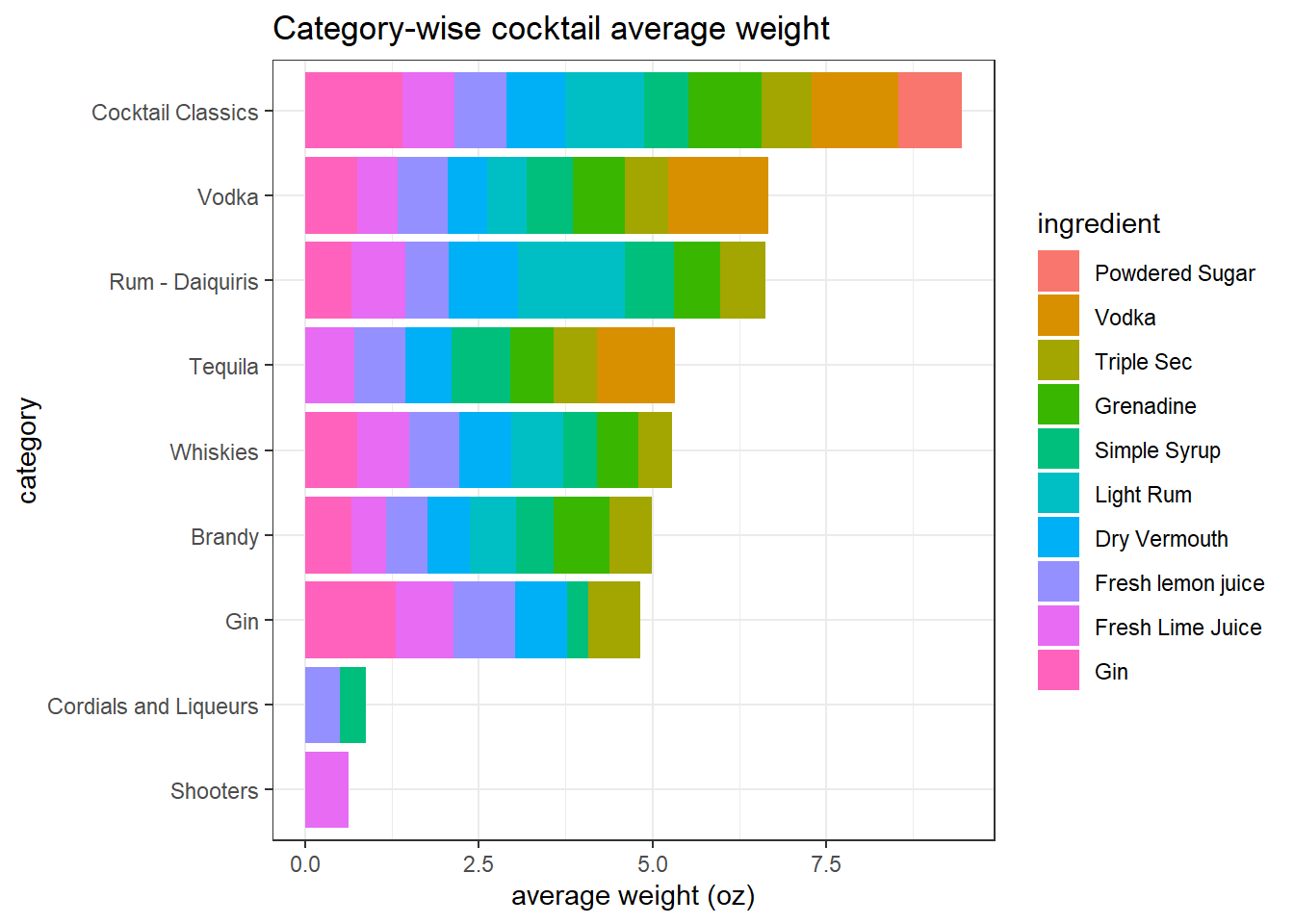

The follwoing graph and PCA sections are followed by my other blog post about Bob Ross, and here is the link.

Graph

set.seed(2022)

boston_cocktails %>%
  add_count(ingredient) %>%
  filter(n >= 10) %>%
  pairwise_cor(ingredient, name, sort = T) %>%
  head(100) %>%
  graph_from_data_frame() %>%
  ggraph(layout = "fr") +
  geom_edge_link(aes(alpha = correlation)) +
  geom_node_point() +
  geom_node_text(aes(label = name), vjust = 1, hjust = 1) +
  theme_void()

PCA

binary_matrix <- boston_cocktails %>%
  mutate(value = 1) %>%
  acast(name ~ ingredient)

norm_matrix <- binary_matrix - colMeans(binary_matrix)
svd_results <- svd(norm_matrix)

tidy(svd_results, "v") %>%
  mutate(ingredient = colnames(binary_matrix)[column]) %>%
  filter(PC < 5) %>%
  group_by(PC) %>%
  slice_max(abs(value), n = 20) %>%
  ungroup() %>%
  mutate(PC = paste("Principal Component", PC),
         ingredient = reorder_within(ingredient, value, PC)) %>%
  ggplot(aes(value, ingredient, fill = value > 0)) +
  geom_col(show.legend = F) +
  scale_y_reordered() +
  facet_wrap(~PC, scales = "free_y") +
  ggtitle("First 4 principal components of the ingredients")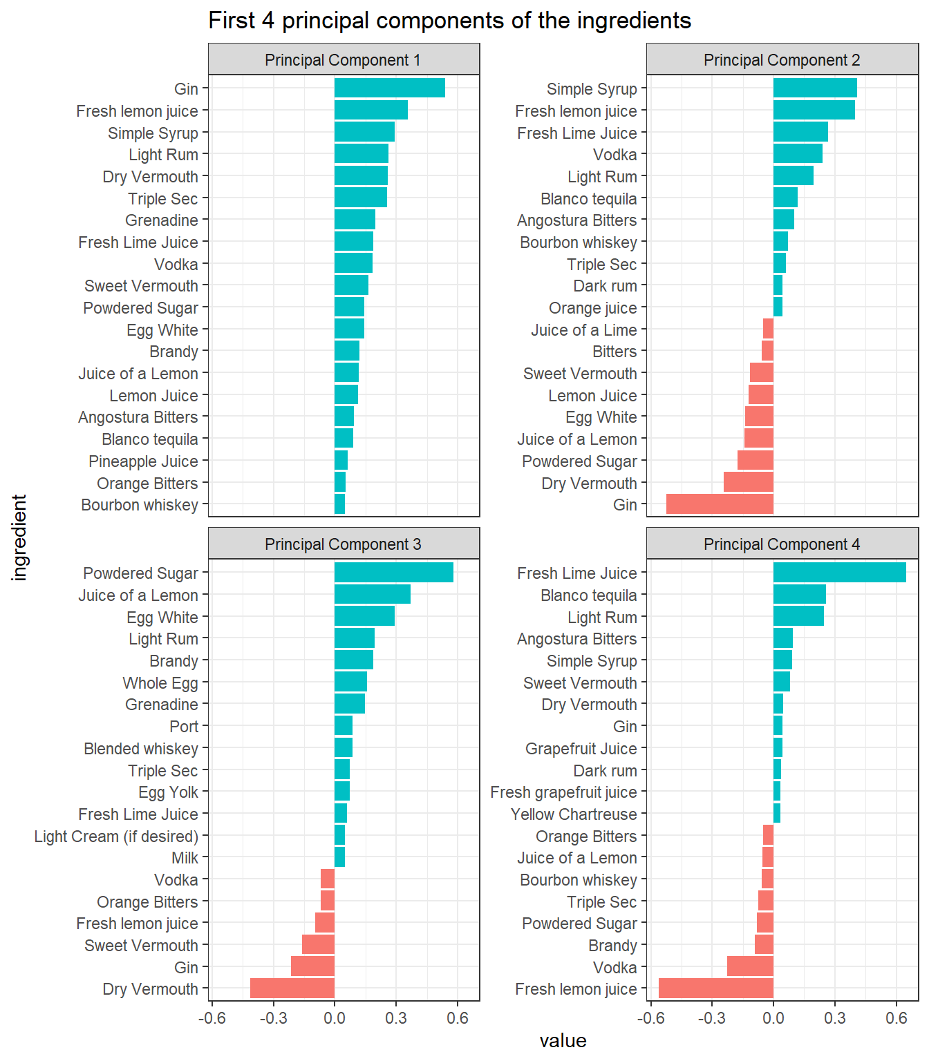

tidy(svd_results, "u")%>%
  mutate(name = rownames(binary_matrix)[row]) %>%
  filter(PC < 5) %>%
  group_by(PC) %>%
  slice_max(abs(value), n = 20) %>%
  ungroup() %>%
  mutate(PC = paste("Principal Component", PC),
         name = reorder_within(name, value, PC)) %>%
  ggplot(aes(value, name, fill = factor(PC))) +
  geom_col(show.legend = F) +
  scale_y_reordered() +
  facet_wrap(~PC, scales = "free_y") +
  ggtitle("First 4 principal components of the cocktail names")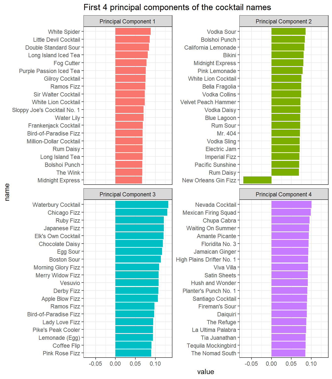

After exploring boston_cocktails and its friend, let's visualize cocktail, which contains more interesting data.

cocktails_oz <- cocktails %>%
  mutate(measure_oz = str_remove(measure, "\\s*oz.*"),
         measure_oz = str_replace(measure_oz, "½", "1/2"), 
         alcoholic = str_to_title(alcoholic),
         category = str_remove_all(category, "\\s*"),
         glass = str_to_title(glass)) %>% 
  filter(!str_detect(measure_oz, "[:alpha:]|\\s")) %>%
  select(-c(id_drink, drink_thumb, iba, video, date_modified)) %>%
  rowwise() %>%
  mutate(measure_oz = round(eval(parse(text = measure_oz)), 2)) %>%
  ungroup()

cocktails_oz %>%
  distinct(drink, .keep_all = T) %>%
  count(category, alcoholic, sort = T) %>%
  filter(!is.na(alcoholic)) %>%
  mutate(category = fct_reorder(category, n, sum)) %>%
  ggplot(aes(alcoholic, category, size = n, color = alcoholic)) +
  geom_point() +
  scale_size_continuous(breaks = seq(0, 400, 50), range = c(2,6)) +
  guides(color = "none") +
  labs(x = NULL,
       y = NULL,
       size = "count",
       title = "Cocktail category and alcohol relations")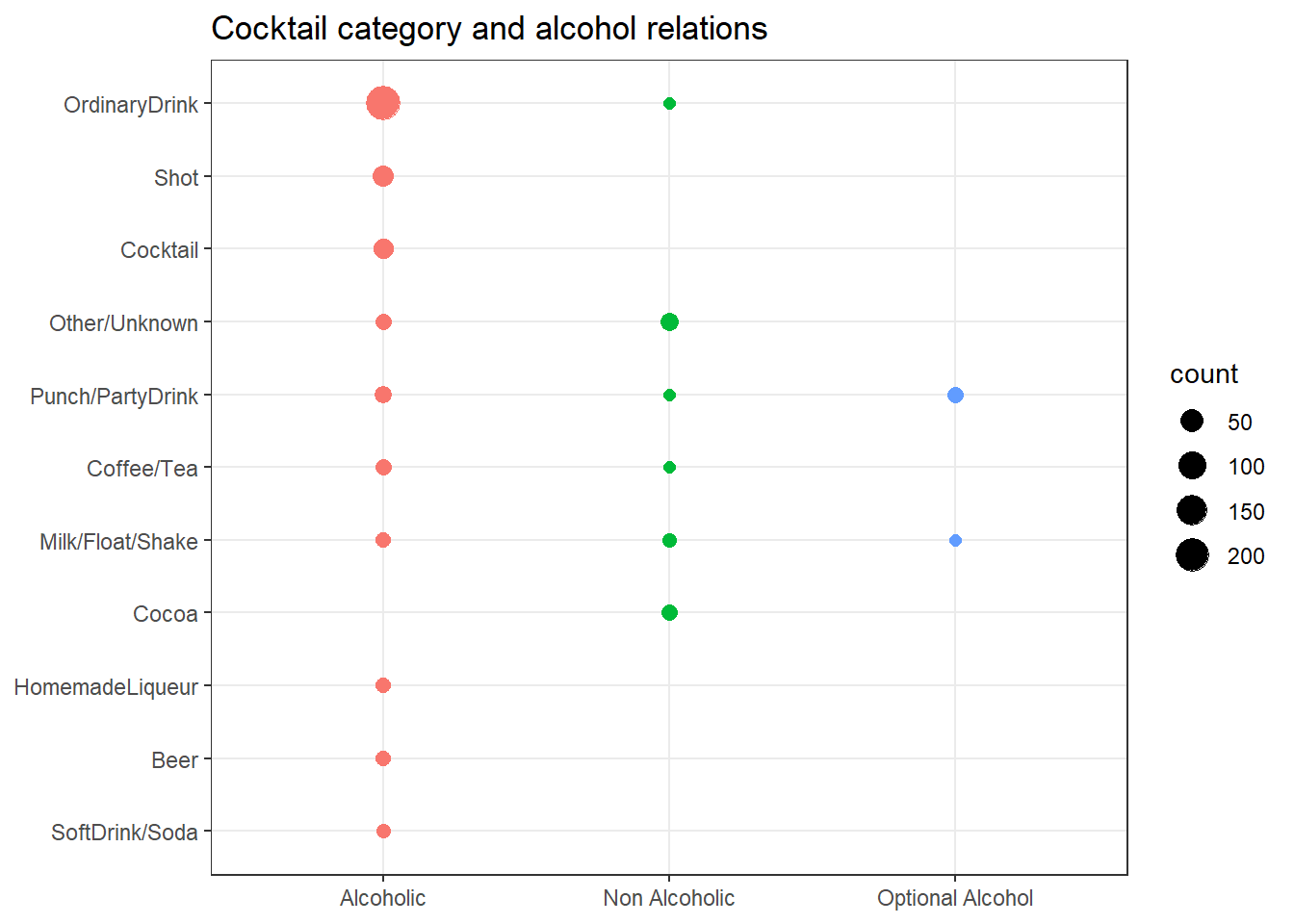

As we can see, most of the cocktails are alcoholic.

Various kinds of cocktails and their weight

cocktails_oz %>%
  group_by(drink) %>%
  mutate(total_weight = sum(measure_oz)) %>%
  ungroup() %>%
  filter(total_weight > 0) %>%
  distinct(drink, alcoholic, category, glass, total_weight) %>%
  filter(total_weight < 20,
         !is.na(alcoholic)) %>%
  mutate(category = reorder_within(category, total_weight, alcoholic, median)) %>%
  ggplot(aes(total_weight, category, fill = category)) +
  geom_boxplot(show.legend = F) +
  scale_y_reordered() +
  facet_wrap(~alcoholic, scales = "free_y", ncol = 1) +
  labs(x = "weight in total (oz)",
       title = "The weight of various cocktails") +
  theme(strip.text = element_text(size = 13),
        plot.title = element_text(size = 18))

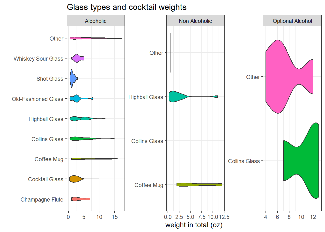
Glass types and the cocktail weights

cocktails_oz %>%
  group_by(drink) %>%
  mutate(total_weight = sum(measure_oz)) %>%
  ungroup() %>%
  filter(total_weight > 0) %>%
  distinct(drink, alcoholic, category, glass, total_weight) %>%
  group_by(drink, glass) %>%
  ungroup() %>%
  filter(total_weight < 20,
         !is.na(alcoholic)) %>%
  mutate(glass = fct_lump(glass, n = 8)) %>%
  ggplot(aes(total_weight, glass, fill = glass)) +
  geom_violin(show.legend = F) +
  facet_wrap(~alcoholic, scales = "free") +
  labs(x = "weight in total (oz)",
       y = "",
       title = "Glass types and cocktail weights")