African-American History Data Visualization (Graph & Word Cloud included)
Thu, Jan 13, 2022
5-minute read
This blog post is a little similar to the previous post I had (you can check it out here). The previous one is about the African-American achievements, but this one is about slave transportation, census data, African names, as well as some important historic events recorded. The data sets are from TidyTuesday.
library(tidyverse)
library(scales)
library(glue)
library(tidytext)
library(patchwork)
library(ggraph)
library(ggwordcloud)
theme_set(theme_bw())
blackpast <- read_csv('https://raw.githubusercontent.com/rfordatascience/tidytuesday/master/data/2020/2020-06-16/blackpast.csv')
census <- read_csv('https://raw.githubusercontent.com/rfordatascience/tidytuesday/master/data/2020/2020-06-16/census.csv')
slave_routes <- read_csv('https://raw.githubusercontent.com/rfordatascience/tidytuesday/master/data/2020/2020-06-16/slave_routes.csv')
african_names <- read_csv('https://raw.githubusercontent.com/rfordatascience/tidytuesday/master/data/2020/2020-06-16/african_names.csv')U.S. and its subregion population in total
census %>%
  group_by(region, year) %>%
  summarize(total = sum(total)) %>%
  ungroup() %>%
  mutate(region = fct_reorder(region, -total, sum)) %>%
  ggplot(aes(year, total, color = region)) +
  geom_line(size = 1) +
  scale_y_log10(labels = comma) +
  scale_x_continuous(breaks = seq(min(census$year), max(census$year), 25)) +
  labs(y = "total population",
title = "Total U.S. and subregion population") 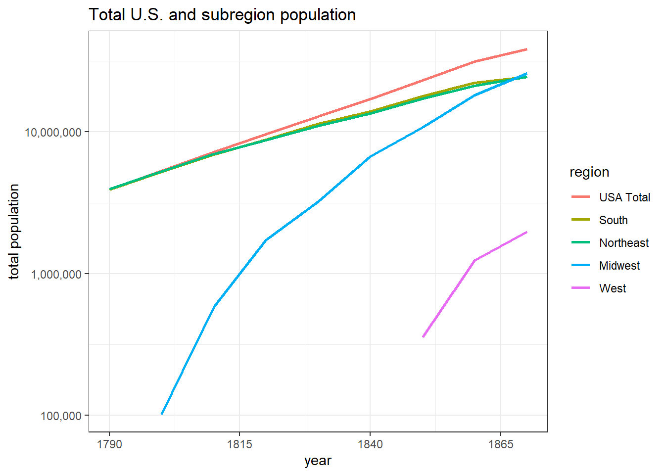
U.S. Population among various races
census %>%
  filter(region == "USA Total") %>%
  select(-division) %>%
  pivot_longer(cols = -c(region, year), names_to = "variable", values_to = "population") %>%
  filter(variable != "total") %>%
  mutate(variable = str_replace(variable, "_", " "),
         variable = str_to_title(variable),
         variable = fct_reorder(variable, -population, sum)) %>%
  ggplot(aes(year, population, color = variable)) +
  geom_line(size = 1) +
  scale_y_log10(labels = comma) +
  scale_x_log10(breaks = seq(min(census$year), max(census$year), 25)) +
  labs(color = NULL,
       title = "The total population across various races of the U.S.") +
  theme(strip.text = element_text(size = 13),
        plot.title = element_text(size = 15))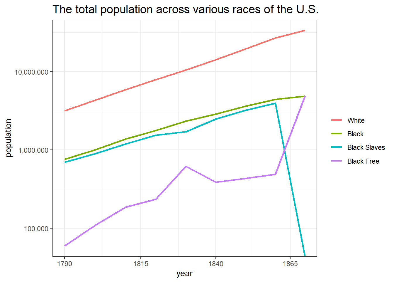
The U.S. population across four different regions
census %>%
  select(-division) %>%
  pivot_longer(cols = -c(region, year), names_to = "variable", values_to = "population") %>%
  filter(region != "USA Total",
         variable != "total") %>%
  group_by(region, year, variable) %>%
  summarize(population = sum(population)) %>%
  ungroup() %>%
  mutate(variable = str_replace(variable, "_", " "),
         variable = str_to_title(variable)) %>%
  mutate(variable = fct_reorder(variable, -population, sum)) %>%
  ggplot(aes(year, population, color = variable)) +
  geom_line(size = 1) +
  facet_wrap(~region) +
  scale_x_log10(breaks = seq(min(census$year), max(census$year), 25)) +
  scale_y_log10(labels = comma) +
  labs(color = NULL,
       title = "The population across four regions of the U.S.") +
  theme(strip.text = element_text(size = 13),
        plot.title = element_text(size = 15))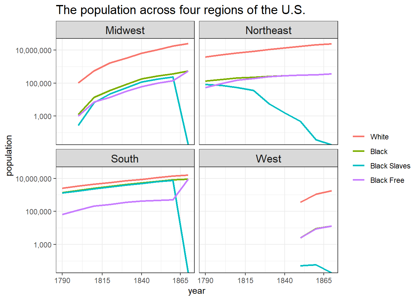
set.seed(2022)
slave_routes %>%
  count(port_origin, port_arrival, sort = T) %>%
  filter(port_arrival != port_origin) %>%
  head(50) %>%
  ggraph(layout = "fr") +
  geom_edge_link(aes(width = n),
                 arrow = arrow(length = unit(4, 'mm'),
                               type = "open")) +
  geom_node_point() +
  geom_node_text(aes(label = name, color = name), hjust = 0.5, vjust = 1, check_overlap = T, size = 5) +
  scale_edge_width_continuous(range = c(1,2)) +
  theme_void() +
  guides(color = "none") +
  labs(edge_width = "# of transports",
       title = "How were slaves being transported between ports?") +
  theme(plot.title = element_text(size = 18))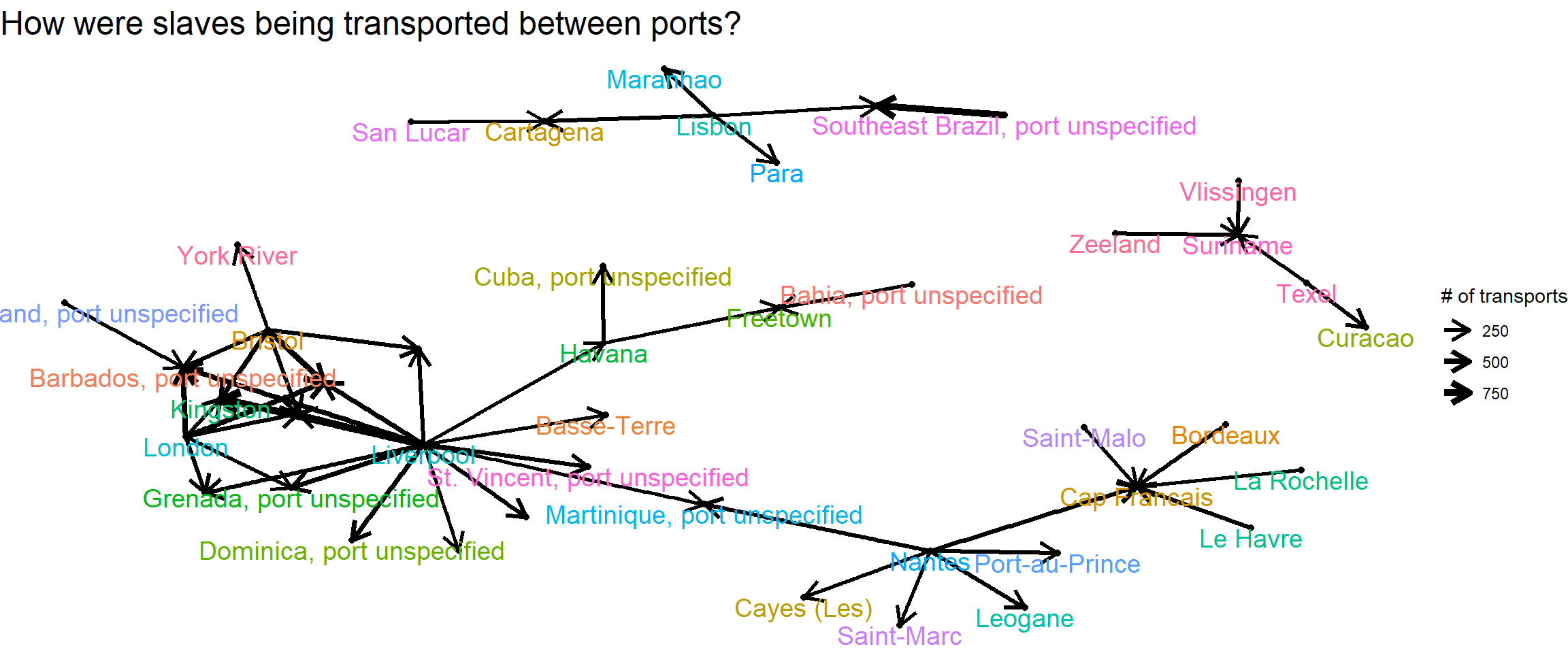
Captains transporting slaves
captains <- slave_routes %>%
  rename(captain_name = captains_name) %>%
  separate_rows(captain_name, sep = "<br/> ") %>%
  filter(!is.na(captain_name)) %>%
  separate(captain_name, c("last_name", "first_name"), sep = ", ") %>%
  mutate(captain_full_name = paste(first_name, last_name))

captains %>%
  count(captain_full_name, sort = T) %>%
  head(20) %>%
  mutate(captain_full_name = fct_reorder(captain_full_name, n)) %>%
  ggplot(aes(n, captain_full_name)) +
  geom_col() +
  labs(x = "# of voyages",
       y = "captain name",
       title = "Top 20 captains on # of voyages of transporting slaves")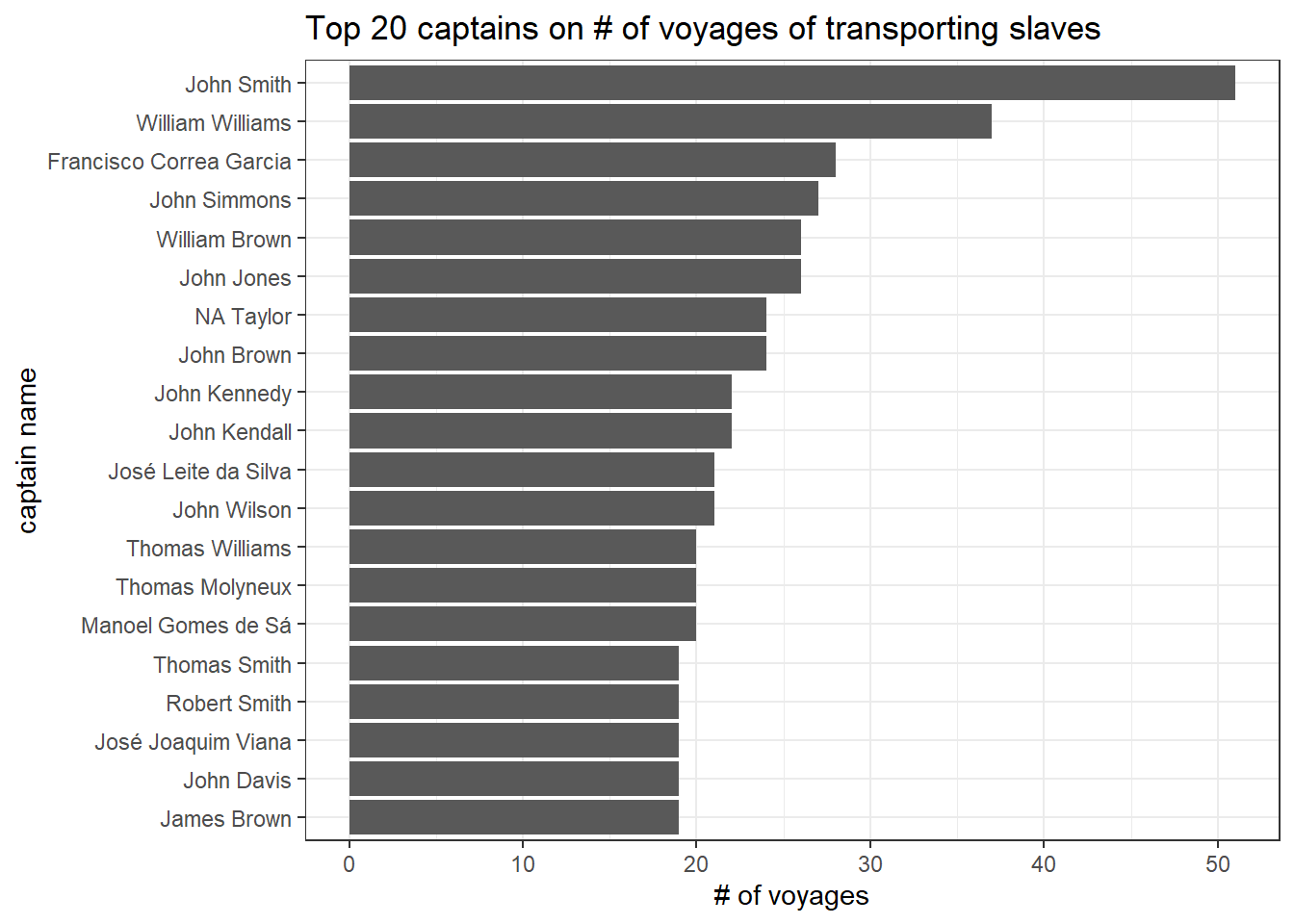
Captains transporting # of slaves
captains %>%
  group_by(captain_full_name) %>%
  summarize(n_slaves = sum(n_slaves_arrived)) %>%
  arrange(desc(n_slaves)) %>%
  head(20) %>%
  mutate(captain_full_name = fct_reorder(captain_full_name, n_slaves)) %>%
  ggplot(aes(n_slaves, captain_full_name)) +
  geom_col() +
  labs(x = "# of slaves being transported",
       y = "captain",
       title = "Top 20 captains transporting most of the slaves")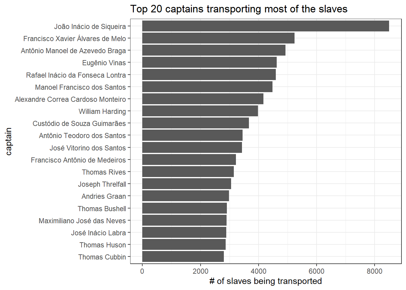
Total # of slaves being transported over the years
captains %>%
  group_by(year_arrival) %>%
  summarize(n_slaves = sum(n_slaves_arrived, na.rm = T)) %>%
  ungroup() %>%
  ggplot(aes(year_arrival, n_slaves)) +
  geom_line(size = 1, color = "pink") +
  scale_x_continuous(breaks = seq(1500, 1900, 50)) +
  labs(x = "arrival year",
       y = "# of slaves in total",
       title = glue("# of slaves arrived being transported from {min(captains$year_arrival)} to {max(captains$year_arrival)}"))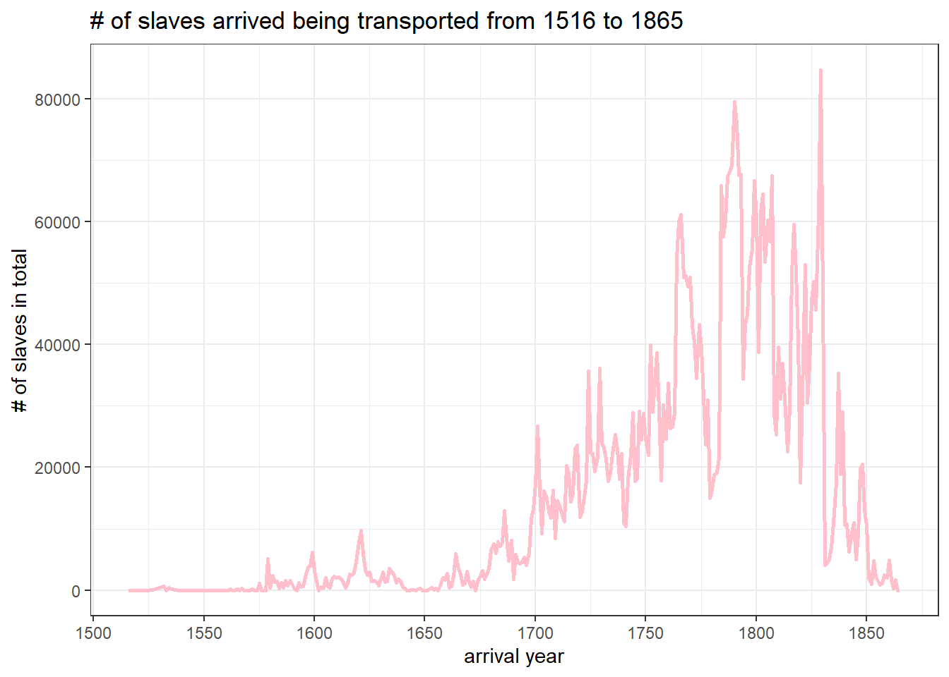
Working on african_names
Overview of age and height
age <- african_names %>%
  mutate(port_disembark = str_remove(port_disembark, " unspecified|,"),
         gender = fct_reorder(gender, age, median, na.rm = T)) %>%
  ggplot(aes(age, gender, fill = port_disembark)) +
  geom_boxplot() +
  labs(y = NULL,
       title = "Slave age and gender")


height <- african_names %>%
  mutate(port_disembark = str_remove(port_disembark, " unspecified|,"),
         gender = fct_reorder(gender, age, median, na.rm = T)) %>%
  ggplot(aes(height, gender, fill = port_disembark)) +
  geom_boxplot() +
  labs(y = NULL,
       title = "Slave height and gender")


age / height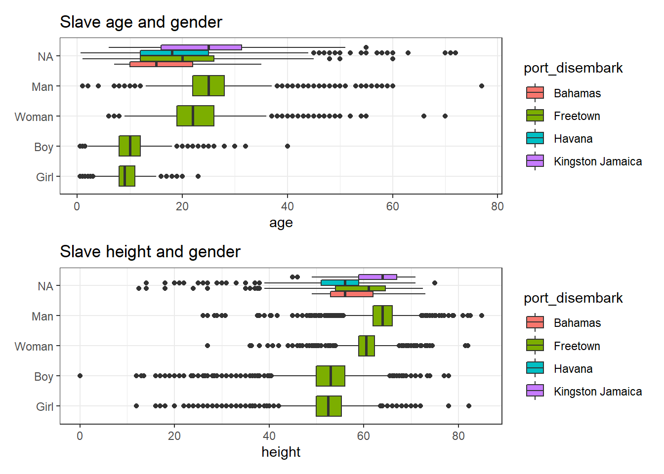
Average age and height
african_names %>%
  group_by(year_arrival, gender) %>%
  summarize(age = mean(age, na.rm = T),
            height = mean(height, na.rm = T)) %>%
  ungroup() %>%
  pivot_longer(cols = c("age", "height")) %>%
  filter(!is.na(gender)) %>%
  mutate(gender = fct_reorder(gender, -value, sum, na.rm = T)) %>%
  ggplot(aes(year_arrival, value, color = gender)) +
  geom_line(size = 1) +
  facet_wrap(~name) +
  theme(strip.text = element_text(size = 13),
        plot.title = element_text(size = 15)) +
  labs(x = "arrival year",
       y = NULL,
       color = NULL,
       title = "Average age and height among all slaves over the years")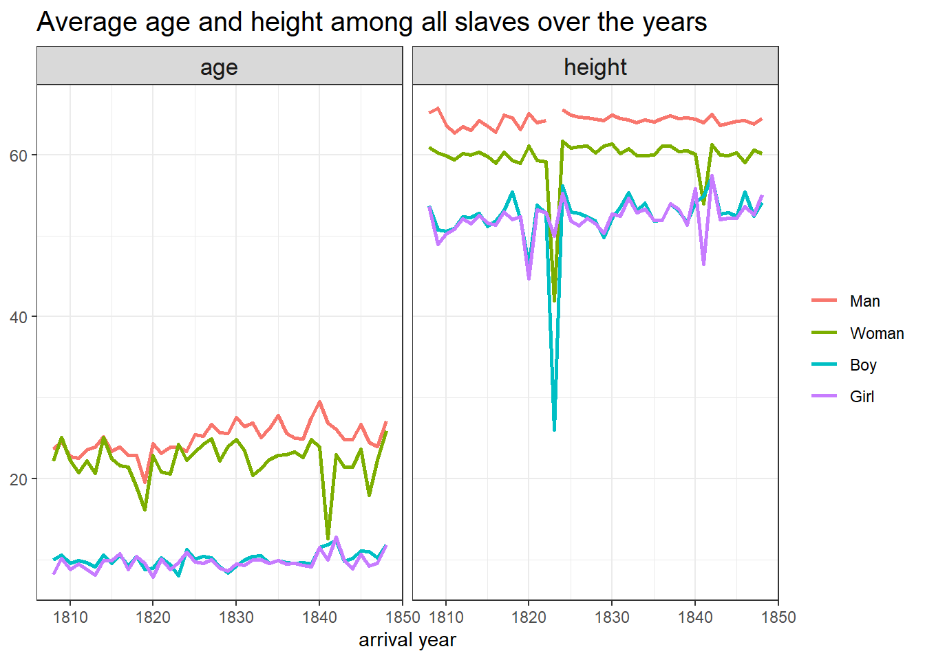
The most popular slave names
african_names %>%
  group_by(gender, name) %>%
  summarize(n = n()) %>%
  ungroup() %>%
  group_by(gender) %>%
  slice_max(n, n = 10) %>%
  ungroup() %>%
  filter(!is.na(gender)) %>%
  mutate(name = reorder_within(name, n, gender)) %>%
  ggplot(aes(n, name, fill = gender)) +
  geom_col() +
  scale_y_reordered() +
  facet_wrap(~gender, scales = "free_y") +
  theme(legend.position = "none",
        strip.text = element_text(size = 13),
        plot.title = element_text(size = 15)) +
  labs(x = "count",
title = "Top 10 most popular names among various groups of slaves") 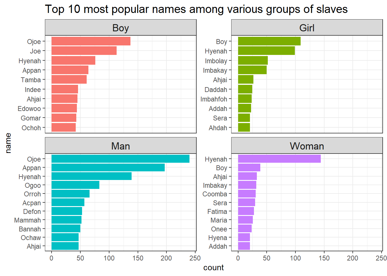
african_names %>%
  group_by(gender, name) %>%
  summarize(n = n()) %>%
  ungroup() %>%
  group_by(gender) %>%
  slice_max(n, n = 30) %>%
  ungroup() %>%
  filter(!is.na(gender)) %>%
  ggplot(aes(label = name, color = gender, size = n)) +
  geom_text_wordcloud_area(show.legend = T) +
  scale_size_area(max_size = 20) +
  theme_minimal() +
  guides(size = "none")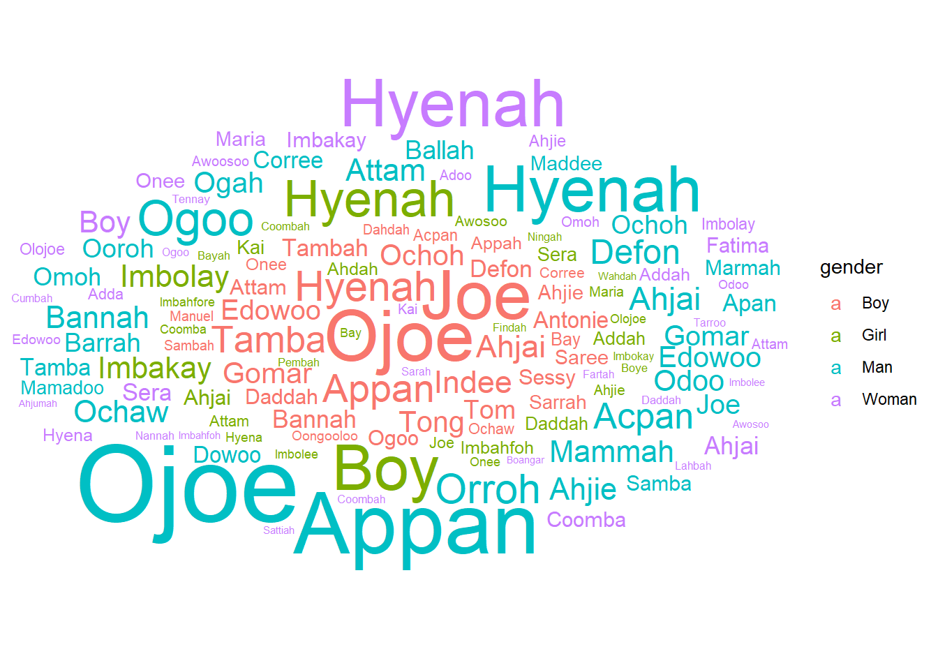
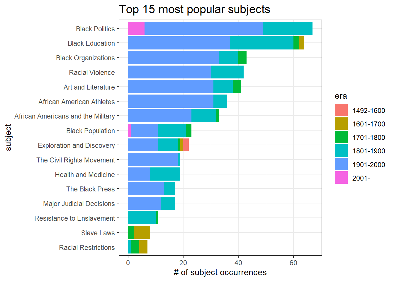
Popular subjects in various eras
blackpast %>%
  mutate(country = str_remove(country, "The ")) %>%
  mutate(subject = fct_lump(subject, n = 15),
         country = fct_recode(country,
                              "United States" = "U.S.",
                              "United States" = "Unied States")) %>%
  filter(subject != "Other",
         country == "United States") %>%
  count(era, country, subject, sort = T) %>%
  mutate(subject = fct_reorder(subject, n, sum)) %>%
  ggplot(aes(n, subject, fill = era)) +
  geom_col() +
  labs(x = "# of subject occurrences",
       title = "Top 15 most popular subjects") +
  theme(strip.text = element_text(size = 13),
        plot.title = element_text(size = 15))