Pretraining a Language Model From Scratch: Argonne 1.0 to 3.0
Contents 9 sections
In an earlier article I described how a small language model can be taught to reason. That discussion rested on a claim worth restating: the capabilities of a fine-tuned model are largely determined by the quality of the underlying base model. The present article turns to that foundation directly — how the base models themselves were built, beginning from nothing more than a corpus of text and a randomly initialized set of parameters.
This was not a single undertaking. Over roughly fifteen months I pretrained a language model from scratch five times, each version a near-complete redesign. The models grew from a modest 276-million-parameter prototype to a 2.9-billion-parameter system, and the hardware beneath them advanced from an eight-GPU node to a smaller, substantially faster configuration. Each version exposed a limitation of the one before it; several of those lessons were expensive.
The most important of them can be stated at the outset: a larger model is not necessarily a better one. The costliest error in this series was training the largest model of the family — the only version never released, because it could not be trained on enough data to justify its size. The version that followed was deliberately smaller, and it was the first I was fully satisfied with.
As in the earlier article, every figure and every quantity reported here is drawn from my own training logs and code. No background in machine learning is assumed.
What pretraining from scratch entails
A brief, non-technical overview will make the remainder self-contained.
A language model predicts the next word — more precisely, the next token, a word or fragment of a word. Given sufficient text, this single objective yields fluent writing. Pretraining is the first and by far the most computationally expensive phase: the model begins as a large array of randomly initialized numbers — its parameters — and is shown an enormous quantity of text, repeatedly predicting the next token and adjusting those parameters slightly at each of billions of steps. The result is a base model: broadly knowledgeable, but not yet able to follow instructions or hold a conversation. (Instilling those behaviours is the subject of the earlier article.)
Two quantities characterize the scale of a base model, and the relationship between them is decisive:
- Parameters — the size of the model, and hence its capacity to store what it learns.
- Tokens — the quantity of text on which it is trained.
A widely cited heuristic, derived from the Chinchilla study, holds that the two should be balanced at approximately 20 tokens of training text per parameter. When tokens are too few relative to parameters, a large model is under-trained and much of its capacity goes unused. This ratio recurs throughout the account that follows.
“From scratch” is meant literally: no pre-existing model and no downloaded starting point — only randomly initialized parameters, raw text, and a considerable amount of computation. The complete family of models is shown below.
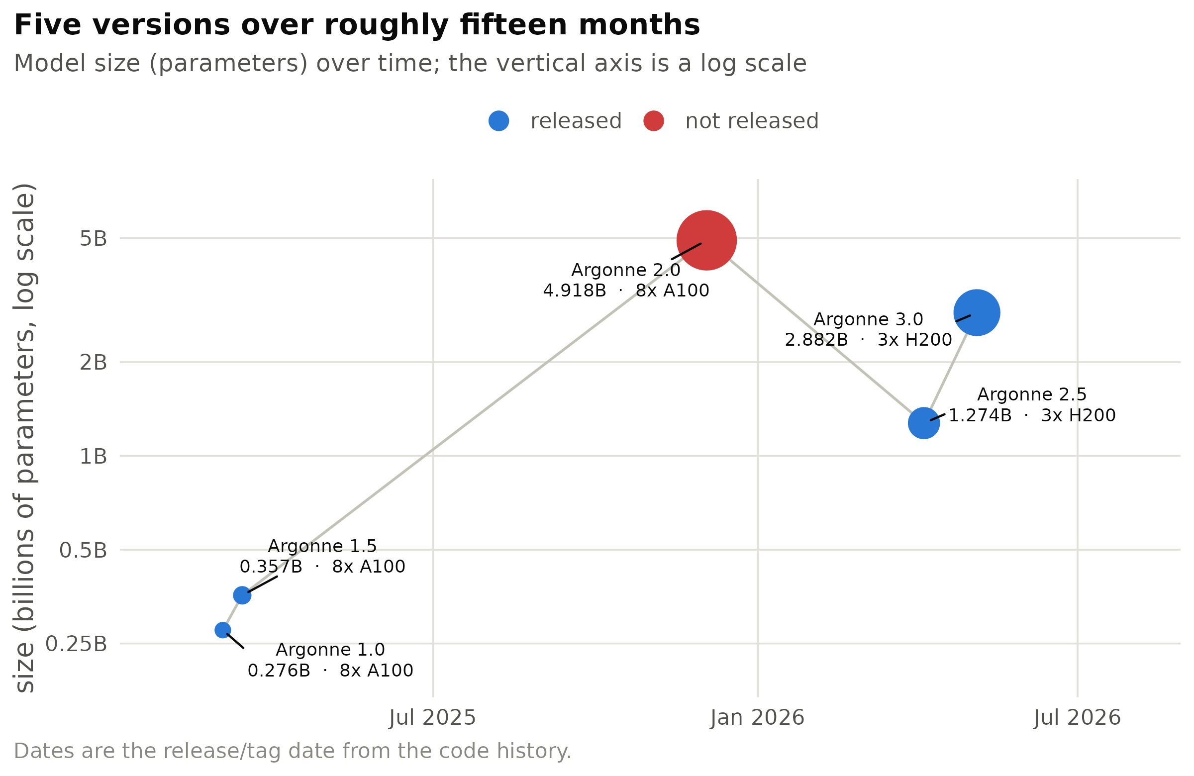
Figure 1: Each version, positioned by release date and parameter count; the vertical axis is logarithmic. Colour indicates release status. Argonne 2.0 (red) was the largest model trained and the only one not released.
The same models are summarized below and are discussed in turn.
| Version | Size | Style | Trained on | Hardware | Released |
|---|---|---|---|---|---|
| 1.0 | 276M | GPT-style | FineWeb-Edu | 8× A100 | Yes |
| 1.5 | 357M | GPT-style | FineWeb-Edu | 8× A100 | Yes |
| 2.0 | 4.9B | modernized | FineWeb (~21.9B tokens) | 8× A100 | No |
| 2.5 | 1.27B | modernized | FineWeb (~76B tokens) | 3× H200 | Yes |
| 3.0 | 2.88B | + stability stack | FineWeb (~76B tokens) → long-context | 3× H200 | Yes |
Argonne 1.0 and 1.5: initial prototypes
The first model was simply called Argonne. It was small — 276 million parameters across 12 layers — and, by current standards, conservative in design: it used the original GPT-2-era components (LayerNorm, a GELU feed-forward network, learned positional embeddings, and standard multi-head attention), together with a purpose-built vocabulary of 12,000 tokens trained on the corpus itself.
It was trained on FineWeb-Edu, an education-oriented, quality-filtered subset of web text.
Training used a single node of eight NVIDIA A100 GPUs and required approximately 1,440
GPU-hours (eight GPUs for roughly a week) over 160,000 optimization steps. Argonne 1.5 followed
eleven days later: the same architecture extended to 16 layers and 357 million parameters, with
the first efficiency improvements — FlashAttention, a faster method of computing attention that
increased the amount of text processed per step by a factor of 2.6, and torch.compile. Both were
released on Hugging Face.
These were proofs of concept, intended to establish whether a coherent language model could be trained end to end on my own hardware and produce fluent English. They could. While not competitive on benchmarks, they validated the training pipeline that every subsequent version would reuse.
An aside: an experiment on the Aurora supercomputer
One early experiment did not lead to a released model but merits mention. In parallel with the A100 work, I ported the trainer to Intel GPUs on Aurora, the flagship supercomputer at Argonne National Laboratory, using an entirely different software stack — Intel’s oneAPI, oneCCL, and MPI in place of NVIDIA’s CUDA — distributed across 32 nodes. There is a certain symmetry in a project named after Argonne running, however briefly, on the laboratory’s own machine.
The port functioned, but it proved a dead end: every released model in this series was ultimately trained on NVIDIA hardware, for which the tooling was more mature and less troublesome for a single developer. This was the first instance of a theme that recurs throughout the hardware history below — the most capable machine available is of little use if its software stack is uncooperative.
Argonne 2.0: the limits of scale
Argonne 2.0 was an ambitious redesign and a substantial increase in scale — 4.9 billion parameters, by far the largest model of the family and larger than every version that would follow. The architecture was modernized comprehensively, replacing the GPT-2-era components with those now standard in contemporary open models: RMSNorm (a simpler, more stable normalization), a SwiGLU feed-forward network, rotary position embeddings (RoPE), grouped-query attention (a more efficient attention variant), and tied input/output embeddings. It also adopted a full 150,000-token vocabulary from the Qwen tokenizer. On paper, it was a thoroughly modern model.
Fitting 4.9 billion parameters across eight GPUs required implementing tensor parallelism, which partitions the computation of each layer across all eight devices so that none need hold the entire model.
The difficulty was data. The model was trained on approximately 21.9 billion tokens — a large figure in isolation, but a small one relative to the model’s size:
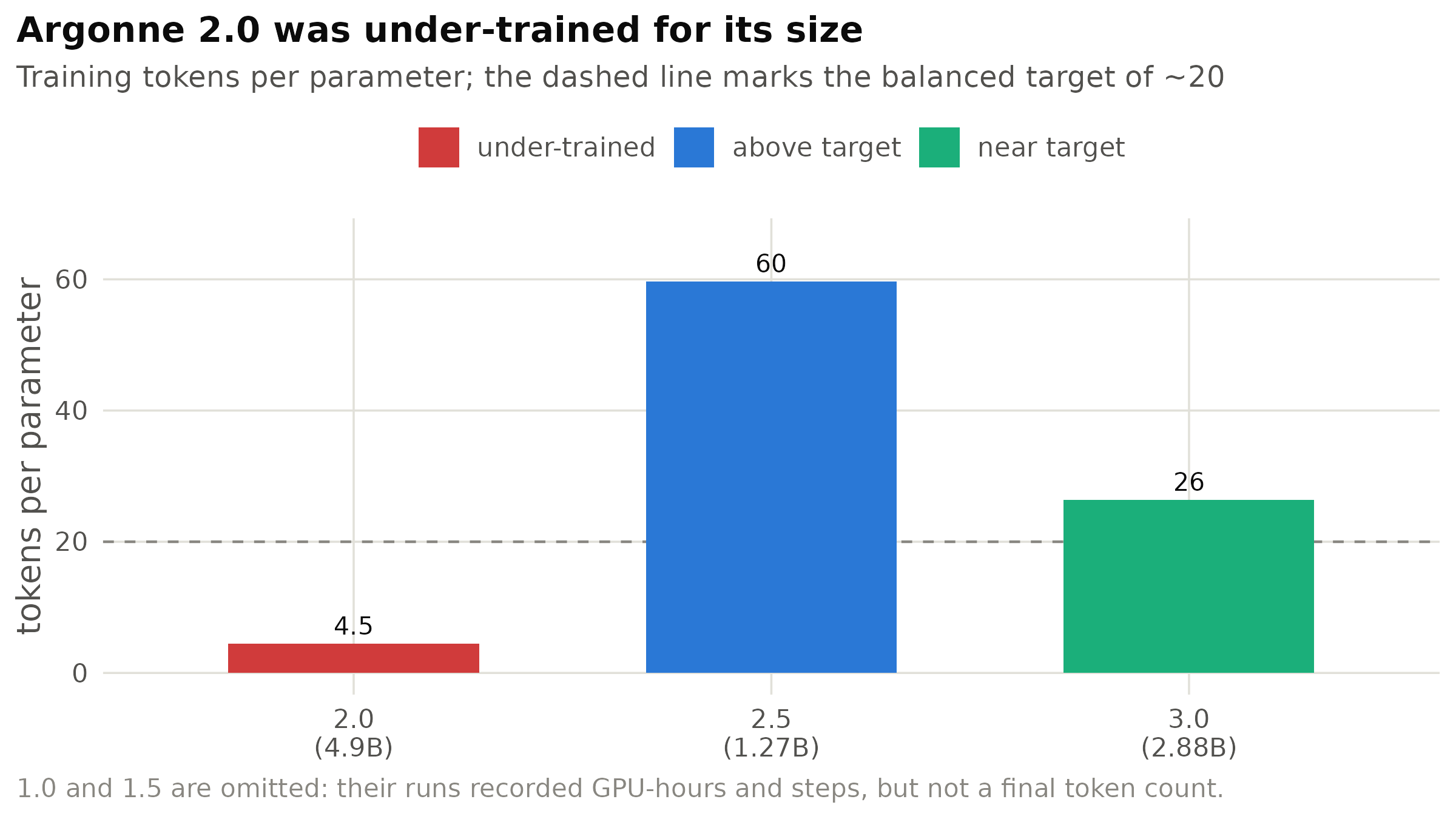
Figure 2: Training tokens per parameter for each model. The dashed line marks the approximate balanced target of 20. Argonne 2.0 was substantially under-trained; the deliberately smaller 2.5 was trained well beyond the target.
At 4.5 tokens per parameter, Argonne 2.0 saw roughly a fifth of the text its capacity warranted, and much of that capacity therefore went unused. Its loss plateaued in the 2.5–3.5 range, and I chose not to release it — a decision I still consider correct. A 4.9-billion-parameter model that could not be trained adequately was, in practice, inferior to a smaller model that could: slower and larger without being more capable. It remains the most expensive effort in this account to produce no public artifact, and the clearest lesson of the project.
Argonne 2.5: correcting course
Argonne 2.5 was a direct response to that error. The model was deliberately reduced in size — to 1.27 billion parameters, roughly a quarter of Argonne 2.0 — and the available compute was redirected toward data. It was trained on approximately 76 billion tokens, or nearly 60 tokens per parameter, making it the most thoroughly trained model in the family. This is the Chinchilla principle expressed in a single version.
Two further changes accompanied 2.5, both concerned with efficiency.
The hardware advanced a generation. The released model was trained on three NVIDIA H200 GPUs on the University of Chicago’s Midway3 cluster; the H200 is considerably newer and faster than the A100 and provides substantially more memory per device. Fewer but newer GPUs outperformed a larger number of older ones.
The training code was greatly simplified. The tensor-parallel and multi-node machinery of 2.0, though powerful, was fragile, and had cost considerable time to failures in cross-GPU communication. For 2.5 I rewrote the trainer as a compact, single-file loop modelled on Andrej Karpathy’s llm.c project. (For the technically inclined: the implementation remained in standard PyTorch; I adopted llm.c’s design principles rather than its C code. The central idea was its data format — tokenizing the entire corpus once, in advance, into a compact binary file that the trainer reads directly from disk.) I first built a more elaborate multi-node variant, combining tensor and data parallelism across several eight-GPU nodes, and then abandoned it: on three capable GPUs, the simpler and more robust approach proved superior. Simplicity was, in this instance, a genuine advantage.
Argonne 2.5 was released as a base model, an instruction-tuned variant, and a long-context variant. It was the first model in the family I considered fully satisfactory.
Argonne 3.0: the production base model
Argonne 3.0 is the current production model and the culmination of the family. It was scaled up again, but conservatively, to 2.88 billion parameters — a size that could be trained thoroughly — and augmented with a set of stability and quality mechanisms built upon the 2.5 design. These are the less conspicuous techniques that keep the training of a large model stable: additional normalization within the attention mechanism (query/key, value, and “sandwich” normalizations), a combination of local and global attention (in which some layers are configured to attend only to nearby tokens), a logit softcap that moderates overconfident predictions, and a longer-range positional encoding. None increases the model’s size; each improves the reliability of training.
Notably, Argonne 3.0 was not a single training run but a sequence of three stages, each building on the last:
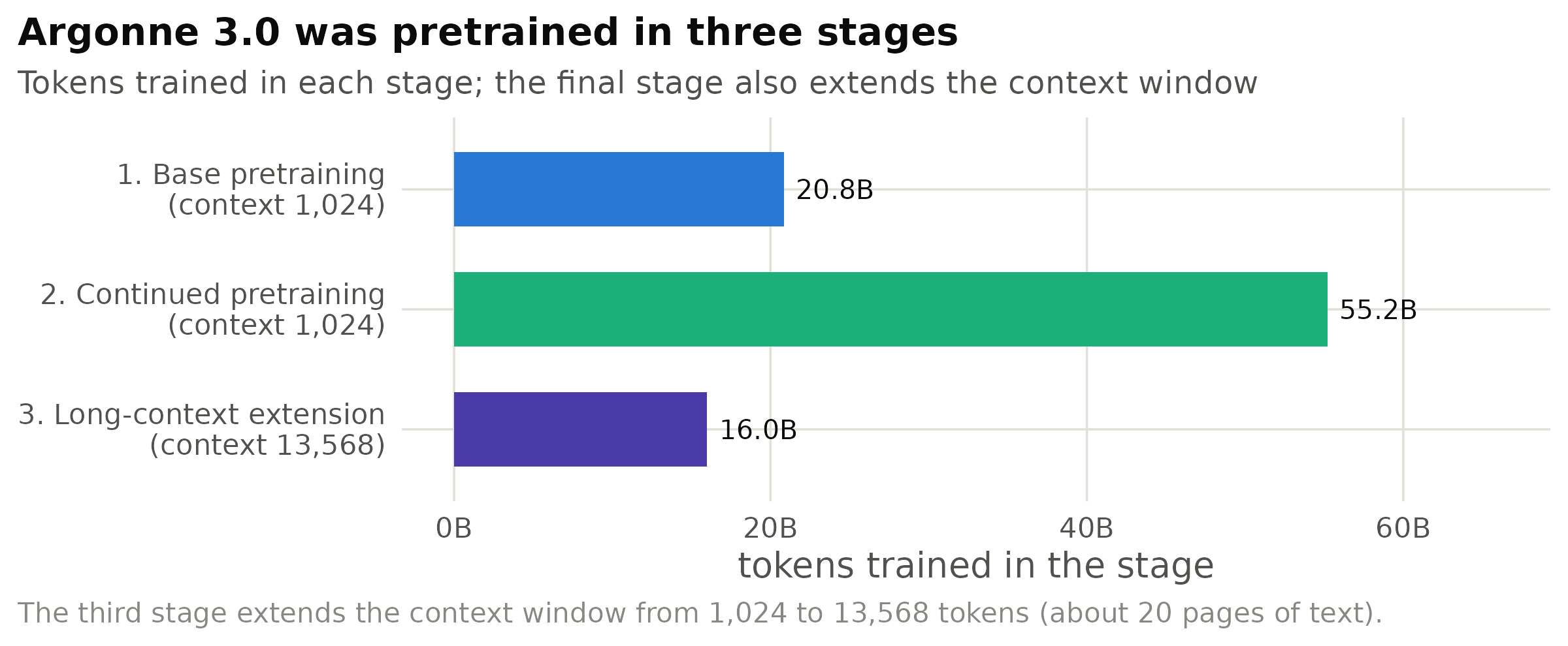
Figure 3: Base pretraining and continued pretraining together comprise ~76 billion tokens (329,148 optimization steps); the long-context stage adds a further 16 billion, for a cumulative total of roughly 92 billion tokens.
- Base pretraining — from random initialization, on approximately 20.8 billion tokens of FineWeb.
- Continued pretraining — the same model trained further on a larger, more recent 55.2-billion-token web crawl, for approximately 76 billion tokens in total.
- Long-context extension — a final 16-billion-token stage on long documents that extended the model’s context window from about 1,000 tokens to 13,568. This stage required a different memory-management scheme (FSDP), as a context of that length does not otherwise fit in memory.
All stages ran on the same three H200 GPUs, in self-resubmitting seven-hour segments — a practical necessity, since a long run must survive the cluster’s time limits, occasional failures, and defective nodes. The base model’s loss settled near 2.5, consistent with expectations for a 2.88-billion-parameter model trained on roughly 76 billion tokens.
One limitation of the resulting base model is worth recording, as it illustrates a general principle. Trained on general web text, Argonne 3.0-base is strong in general knowledge but weak at arithmetic: on a simple 20-question test it answered only 3 correctly, while scoring 14 of 15 on general knowledge. A base model’s abilities are bounded by the composition of its training data, and this particular weakness is what motivated the instruction-tuning and reasoning work described in the companion article. Argonne 3.0-base and its long-context counterpart are the models on which that work was built.
Architectural evolution across versions
Viewed across the family rather than within a single model, a clear progression of modernization emerges: nearly every component was, at some point, replaced by a newer and better-behaved alternative.
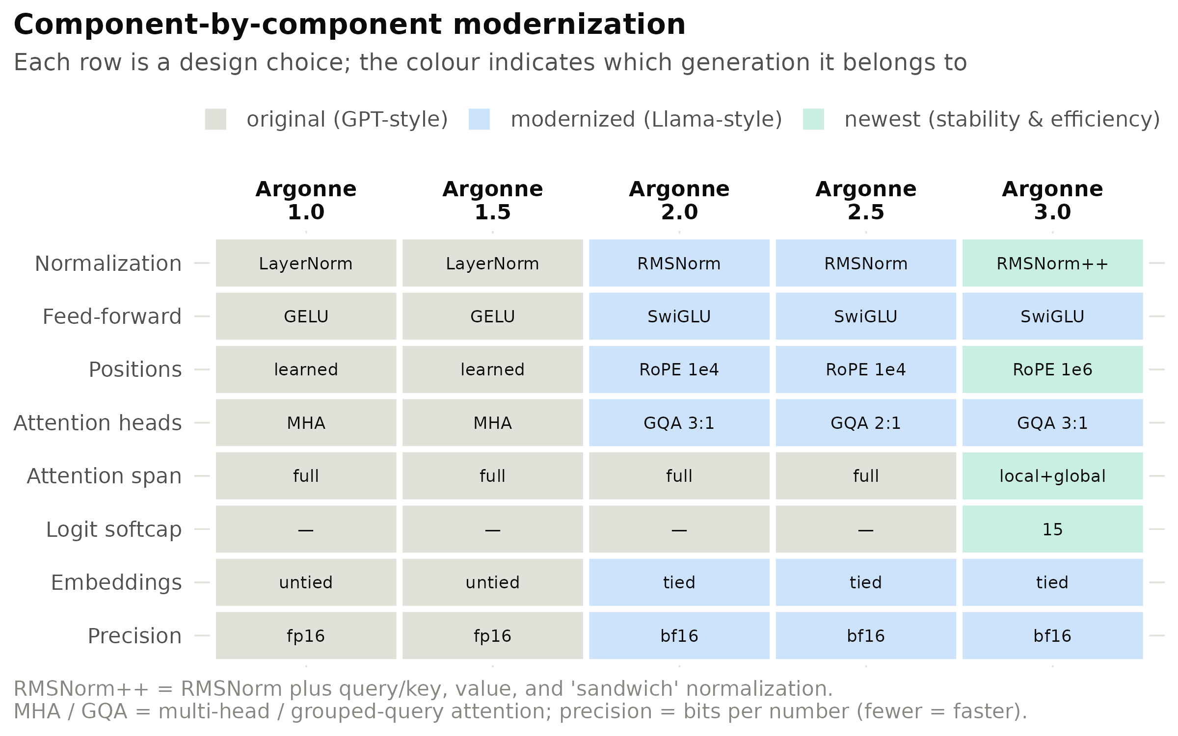
Figure 4: Grey denotes the original GPT-2-era choice; blue, the modern (Llama-style) replacement; green, the most recent stability and efficiency features. The progression runs from left to right across versions.
The pattern merits comment. The architectural changes were front-loaded: the principal modernization occurred at 2.0 and was largely complete by 3.0, after which refinement focused on stability rather than novelty. What continued to matter beyond the architecture was the hardware on which the models were trained — the subject of the final section.
Hardware and systems
Beneath all five versions lies a second line of development: the computing platform. This proved as consequential as any architectural change, since it determined how large a model could be trained adequately.
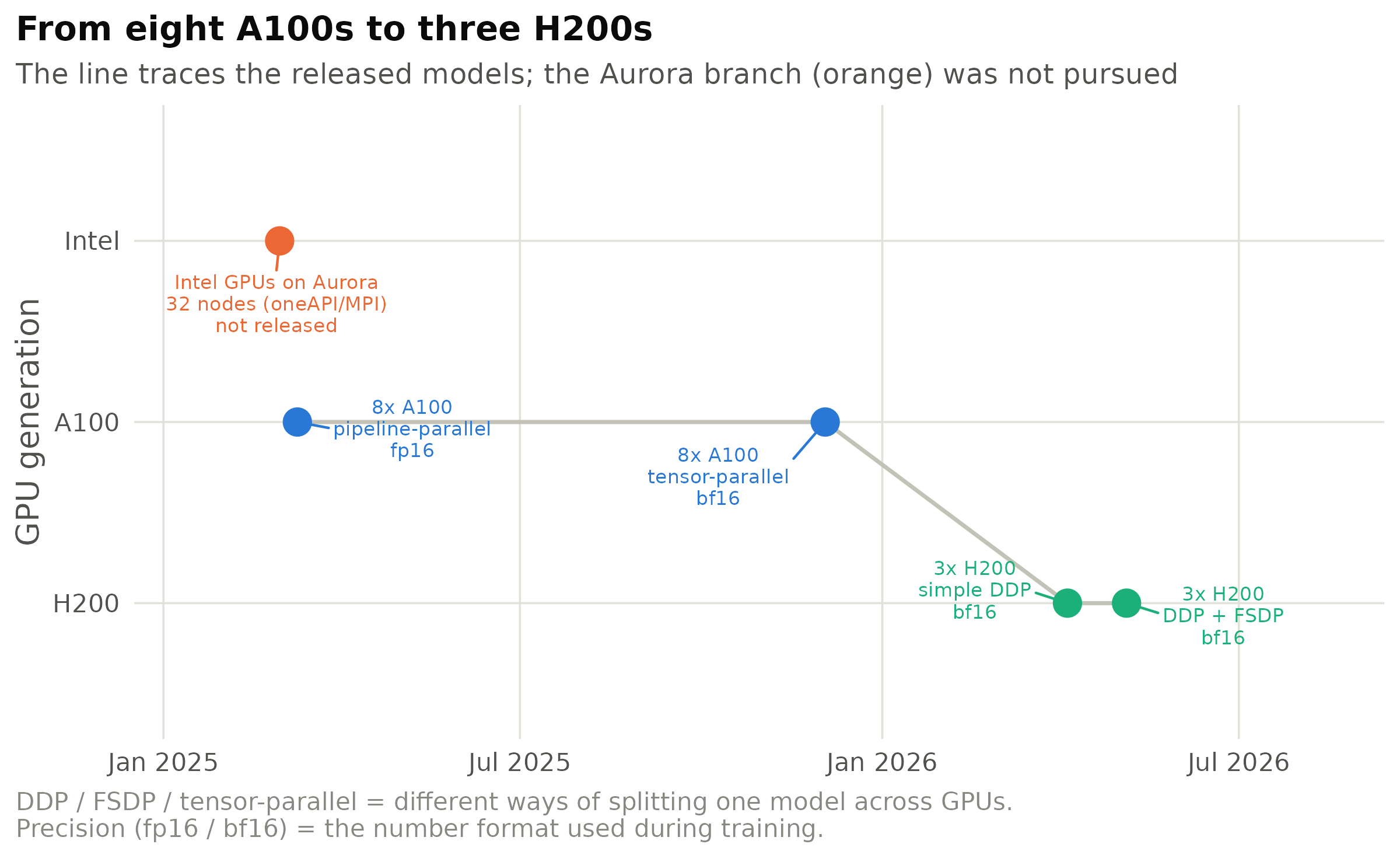
Figure 5: Each point is an era; the label gives how the work was distributed across GPUs and the numerical precision used. The released models progressed from eight A100s to three newer and faster H200s.
Three observations summarize the hardware history:
- Fewer, newer GPUs proved superior. The A100 era used all eight GPUs of a node, together with elaborate partitioning, to accommodate a large model. The H200 era used only three GPUs with the simplest configuration, and trained larger models more quickly. A generational improvement in hardware outweighed a great deal of software complexity.
- The distribution strategy was deliberately simplified — from tensor parallelism, to multi-node schemes, and finally back to straightforward data-parallel training, in which each GPU holds a complete copy of the model and the devices periodically average their updates. The sole exception is the long-context stage of 3.0, which retained a memory-sharing scheme (FSDP) because a 13,568-token context does not otherwise fit.
- Numerical precision was refined from 16-bit floating point (fp16) to the more stable bf16 format, which became standard from Argonne 2.0 onward and improved training stability at no cost in quality.
Lessons
- Model size must be matched to available data. The one model I oversized (2.0, at 4.9 billion parameters) was the one never released. The relevant quantity is tokens per parameter, not the parameter count alone.
- The composition of the training data bounds a model’s abilities. Argonne 3.0-base, trained on general web text, was strong in general knowledge but weak at arithmetic (3 of 20). Such limits are set during pretraining and cannot be fully corrected afterward without the right foundation.
- Newer hardware outperforms more hardware. Three H200s in a minimal configuration outperformed eight A100s with elaborate parallelism. Upgrading the hardware is often preferable to complicating the software.
- Simplicity is a feature. Each attempt at more sophisticated distributed-training machinery (multi-node schemes, combined tensor and data parallelism) cost more in failures than it returned in speed. The version ultimately released used the simplest trainer.
- Operational engineering determines whether long runs finish. Self-resubmitting jobs, checkpointing before timeouts, excluding faulty nodes, and tokenizing the data once in advance are unglamorous individually, but collectively they distinguish a run that completes from one that fails partway through.
Availability
The released models and all associated code are publicly available:
- Models: the Argonne family on Hugging Face —
including
argonne-3.0-base, the long-contextArgonne3.0-ctx13568, andArgonne2.5-base. - Code: github.com/PursuitOfDataScience/ArgonneAI — the complete training pipeline, with one branch per version.
- Companion article: the account of what follows pretraining — instruction tuning and reasoning — appears in the earlier article, How I Taught a Small Language Model to Reason.
Across five versions, the recurring lesson is also the least dramatic: the improvements that mattered came from training on well-chosen data and from keeping the system simple — far more than from increasing the model’s size or the sophistication of the code.