slurmwatch: Live Telemetry for HPC Jobs
Contents 5 sections
slurmwatch is an open-source command-line tool that shows what a running job is actually doing to the hardware it was given. Point it at a job — or run it with no arguments and let it find the job itself — and it displays, live in the terminal, the processor time, the memory, and, where the machine has them, the graphics-card activity belonging to that job.
It exists because that information is otherwise surprisingly hard to get. On a high-performance computing (HPC) system one does not own a machine; one requests one. The scheduler grants the request, starts the program, and records how long the allocation was held. What it never records is whether the hardware was used. A job that reserves four processors and ninety-six gigabytes for nine hours while touching one processor and seven gigabytes, and a job that uses everything it asked for, look identical from the queue. Both exit successfully. Both produce output. Only one was worth the allocation.
pip install slurmwatch # or: uv tool install slurmwatch / pipx install slurmwatchslurmwatch 12345 # watch a specific job
slurmwatch # or find your running job automatically
sw 12345 # 'sw' is a short alias for the same command
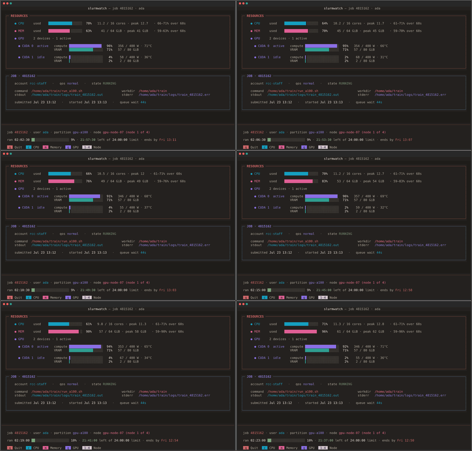
It needs Python 3.10 or later on Linux and depends on just two packages: textual for the interface
and pynvml for the graphics-card readings. GPU monitoring switches itself on where a card is present
and off where there is none, so one installation serves ordinary and accelerated machines alike. On a
processor-only job the dashboard is simply the processor and memory half. The licence is MIT.
This article describes the package, then presents the evidence that motivated it: a set of real jobs that quietly failed to use what they were given. A closing section takes up a question the reader may be holding throughout — why an instrument this mundane should still be necessary in an era of extraordinarily capable AI systems.
Every number below comes either from the tool’s own source and tests, or from measurements recorded during a long machine-learning project on an HPC system. No background in high-performance computing is assumed.
A few terms
- Slurm is the scheduler that hands out an HPC system’s machines. You submit a job — a script
plus a request for resources (
--cpus-per-task=4,--mem=32G, perhaps--gres=gpu:1, and a time limit) — and wait in a queue until those resources are free. - A compute node is the machine your job eventually runs on. You submit from a separate login node and, in the normal course of things, never look at the compute node at all.
- A cgroup (“control group”) is the Linux facility Slurm uses to fence a job in. It is also the authoritative record of what the job consumed.
- A job’s working set is the memory it genuinely needs. It is smaller than the memory the kernel shows it holding, because the kernel also keeps a page cache of recently read file contents on the job’s behalf — memory it can hand back the instant anything else wants it.
- GPU memory (high-bandwidth memory, or HBM) is the memory attached to a graphics card. For machine-learning work it is usually the scarce resource: an 80-gibibyte H100 has about 84.9 GB of it.
- NVML is NVIDIA’s management library, the interface behind the familiar
nvidia-smicommand. It reports each card’s activity, memory, power draw, temperature, and any reason its speed is being held down.
One structural fact drives everything that follows: the cgroup and NVML both live on the compute node, and you do not. The only artefact that ordinarily comes back is a log file containing whatever the program chose to print. Slurm’s own accounting reports coarse, delayed, job-wide totals, and no graphics-card readings at all. The measurements that would answer “is this job using what I asked for?” exist continuously, a few hundred metres away, and are simply never read.
What slurmwatch reports
Your job, not the machine
The central design decision is that slurmwatch reports your job, not the node. Where a machine is
shared with other people’s work, that is the difference between a useful number and a meaningless
one: htop and nvidia-smi show the whole machine, so a neighbour’s memory-hungry program inflates
everything you see. slurmwatch finds your job’s own processes and counts only those.
The obvious source for this is often missing. On the system these measurements come from, the compute nodes keep no per-job processor accounting at all, so the tool falls back to adding up each process by hand — a path checked against Slurm’s own accounting at 1,705 seconds of processor time against its 1,706. The running total only ever climbs, so a short-lived helper process that finishes between two readings cannot erase its work from the tally.
Alongside current usage, the dashboard tracks peak cores in use: the most processors ever busy at
one moment since monitoring began. The kernel offers no such counter, so the tool keeps the running
maximum itself. That is the number to size --cpus-per-task against.
Memory: what the job needs, not what the kernel is holding
The tool separates two memory figures that are constantly confused, and the confusion has cost real jobs real hours.
- The lifetime total is the kernel’s own high-water mark, and it counts the page cache. For a job that reads a large dataset from disk, it reads far above anything the job actually needs.
- The working set leaves the cache out. This is the figure to size
--memagainst, and slurmwatch tracks its running maximum.
The gap is not academic. On a data-preparation job — ordinary processor work, no graphics card involved — Slurm reported a peak of fifteen to eighteen gibibytes, while the real figure was about ten. The request came down from forty-eight gigabytes to twelve on that evidence. The error also runs the other way: a training job that sat steadily at 5.42 GiB was given eight, and was killed at exactly one hour and two minutes. That was its first hourly save, which briefly builds a second copy of the model in memory and peaked at 10.95 GiB. Neither number can be inferred from the other; both are visible live.
A guard turns the memory row amber at eighty-five per cent of the limit and red at ninety — one of only two places in the interface where a colour makes a claim about health rather than simply naming a resource.
Graphics cards, where there are graphics cards
For each card the job holds, slurmwatch reports activity, memory used against the card’s total, power draw against the card’s enforced limit, temperature, and any reason the card is being slowed down. That last pair matters more than it sounds. A card sitting right at its power limit is working hard and perfectly healthy; a card drawing forty per cent of its limit while reporting a hardware slow-down is broken. Without both numbers the two look the same.
Three further distinctions exist because getting them wrong produced a wrong answer:
- A card that is idle but still holding memory is flagged. Before crediting activity to your job, the tool checks that your job owns most of the memory in use — so a neighbour’s work on a shared card is never counted as yours.
- A reading that failed is never printed as a measurement. Zero is a perfectly plausible value for power, temperature, or memory, so each carries a “was this actually readable?” flag. Without them, a card that declined to answer was drawn as an unpowered, sub-freezing device at “0 W, 0 °C” — and, worse, a card that was ninety-nine per cent busy could be scored idle and reported as “0% memory”, which is exactly the figure someone would then size their work against.
- Each card is labelled by the number your own code uses. The number
nvidia-smiprints and the number your program callscuda:0agree only on systems that hide other jobs’ cards from you. Elsewhere they differ, and labelling your cards with the wrong one names devices your code never addresses.
For jobs using several cards at once, the tool also reports how those cards are wired together and how much data is moving between them — useful when the cards are fast but the link between them is not.
Jobs that have not started yet
A queued job has no machine, no cgroup, and no measurements, so pointing a monitoring tool at one might reasonably produce an error. Instead slurmwatch answers the three questions people actually have while waiting: why it is queued, in plain English rather than a Slurm status code; when the scheduler expects it to start, and its place in the queue; and where it could run right now — including the exact command to move it somewhere that fits.
That last part is real analysis rather than a listing. It works out which queues the account may actually use, adds up what is free in each, and names the specific obstacle — machines, processors, memory, or the time limit — for the ones that do not fit. It also declines to advise when advice would be wrong: if a job is held back by an account limit rather than by a shortage of hardware, moving it elsewhere cannot help, and the tool says so instead of suggesting it.
Using it from a script
The dashboard is the visible half of the tool. The other half is built for scripts, monitors, and automated agents.
slurmwatch --once --json 12345      # one snapshot, machine-readable, then exit
slurmwatch --once 12345             # the same snapshot as CSV
slurmwatch --log run.jsonl 12345    # run headless, stream readings to a file
The JSON snapshot carries everything the dashboard shows, and is emitted in strictly standard form so
that ordinary tools such as jq parse it without special handling. The CSV path escapes text fields
that begin with =, +, -, or @, because a job name is arbitrary user input and a spreadsheet
would otherwise treat it as a formula.
The tool attaches from a login node or from the compute node itself. From a login node it reads what Slurm can reach and, where it cannot reach the machine at all, falls back to a summary — clearly labelled, because those figures are lifetime totals for the whole job and must not be mistaken for live readings. Graphics-card measurements require being on the machine, and the interface says which situation it is in rather than quietly reporting no cards.
Three commitments
Facts before verdicts. The dashboard presents measurements. Colour names a resource rather than grading it, with two deliberate exceptions: the memory guard and the card’s idle/active word. The tool does not tell you your job is bad; it tells you what your job is doing. As the next section shows, low usage is sometimes exactly right, so this is accuracy rather than modesty.
Automatic behaviour over flags. With no arguments it finds your running jobs and, if there are several, offers a list. Graphics-card monitoring switches on when there is a card. The output format follows the file extension. The whole option list is ten flags long, and the common paths need none of them.
Honesty about what cannot be read. The code repeatedly refuses to present a failed reading as a measurement. Every one of those guards exists because its absence produced a confidently wrong number during testing.
The package is about 11,800 lines of typed Python against roughly 12,600 lines of tests — 667 test functions, run automatically on four Python versions. The proportion is deliberate. A monitoring tool that is wrong is worse than no tool at all, because its user stops checking.
Why the numbers are worth having
What follows is the evidence: measurements from a long machine-learning project, and the reason the tool was written rather than a feature list justified after the fact.
One term recurs. Training a model proceeds in steps, each step being a single small update to the model. Seconds per step is therefore the basic unit of training speed, and the honest measure of whether a change helped.
Processors and memory are misjudged constantly
The least glamorous failure is the most common, and it has nothing to do with graphics cards. A job asks for processors and memory; nobody ever checks what it used.
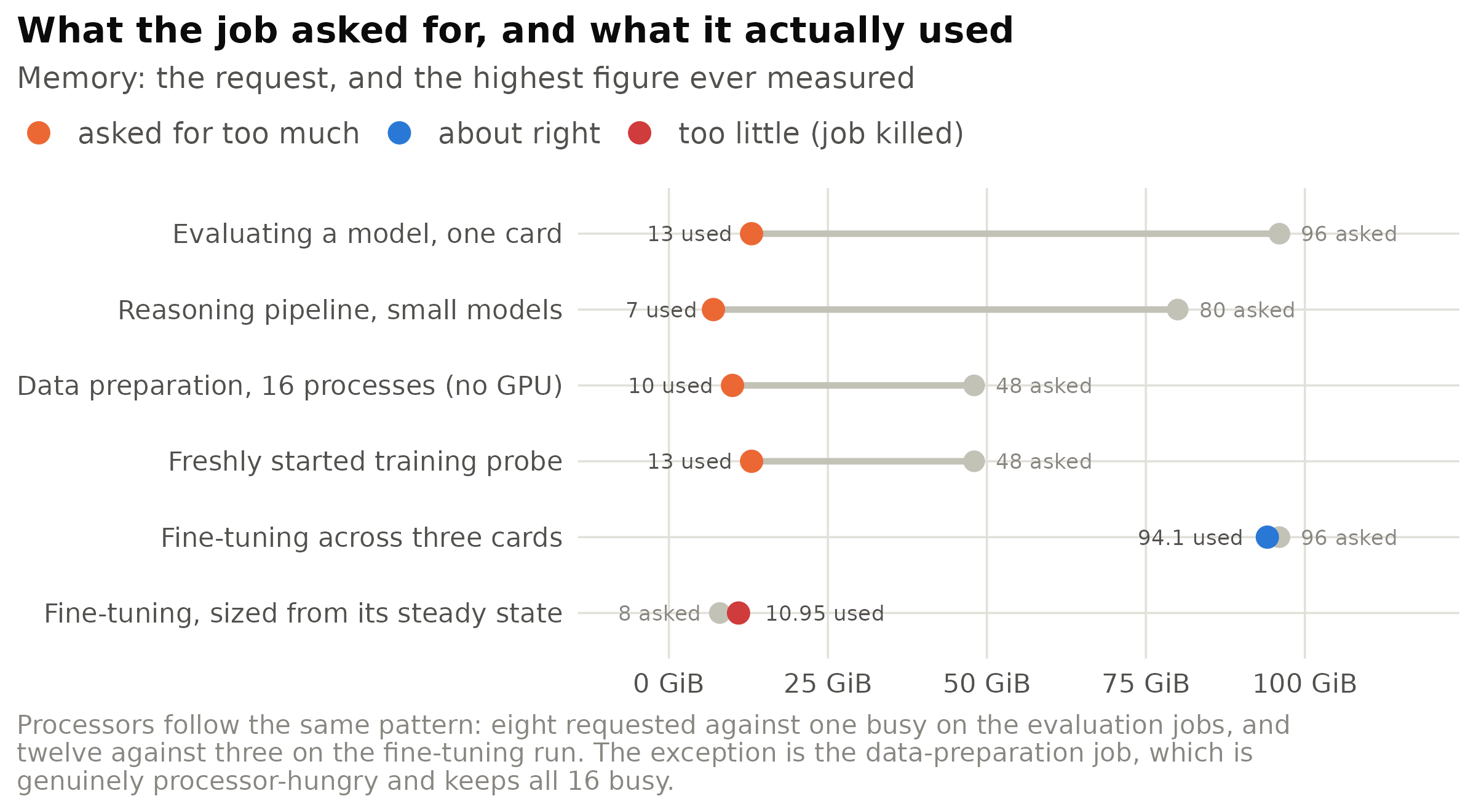
Figure 1: What six real jobs requested, and what they actually needed. Grey marks the request; the coloured point is the measured peak. Four asked for far too much — one by a factor of eleven — which delays the job in the queue and idles memory other work could use. One was right. One asked for too little and was killed for it: the size had been taken from the job’s steady state, an hour before its first save doubled the requirement.
Three points follow. Asking for too much is not free — a job requesting ninety-six gigabytes it will never touch waits longer in the queue and blocks memory other work could use. Asking for too little is worse, and the failure arrives late: the killed job had run normally for an hour before its first save pushed it over. And the right number cannot be reasoned out; it can only be obtained by watching the job through at least one full cycle of whatever it does periodically.
The utilization standard, and how often it was missed
Where a project does use graphics cards, the same problem returns with more money attached. This project ran under a standing rule: every card should be filled to about ninety per cent of its memory. The rule is a rough proxy — a point I return to shortly — but it is concrete and checkable in one command.
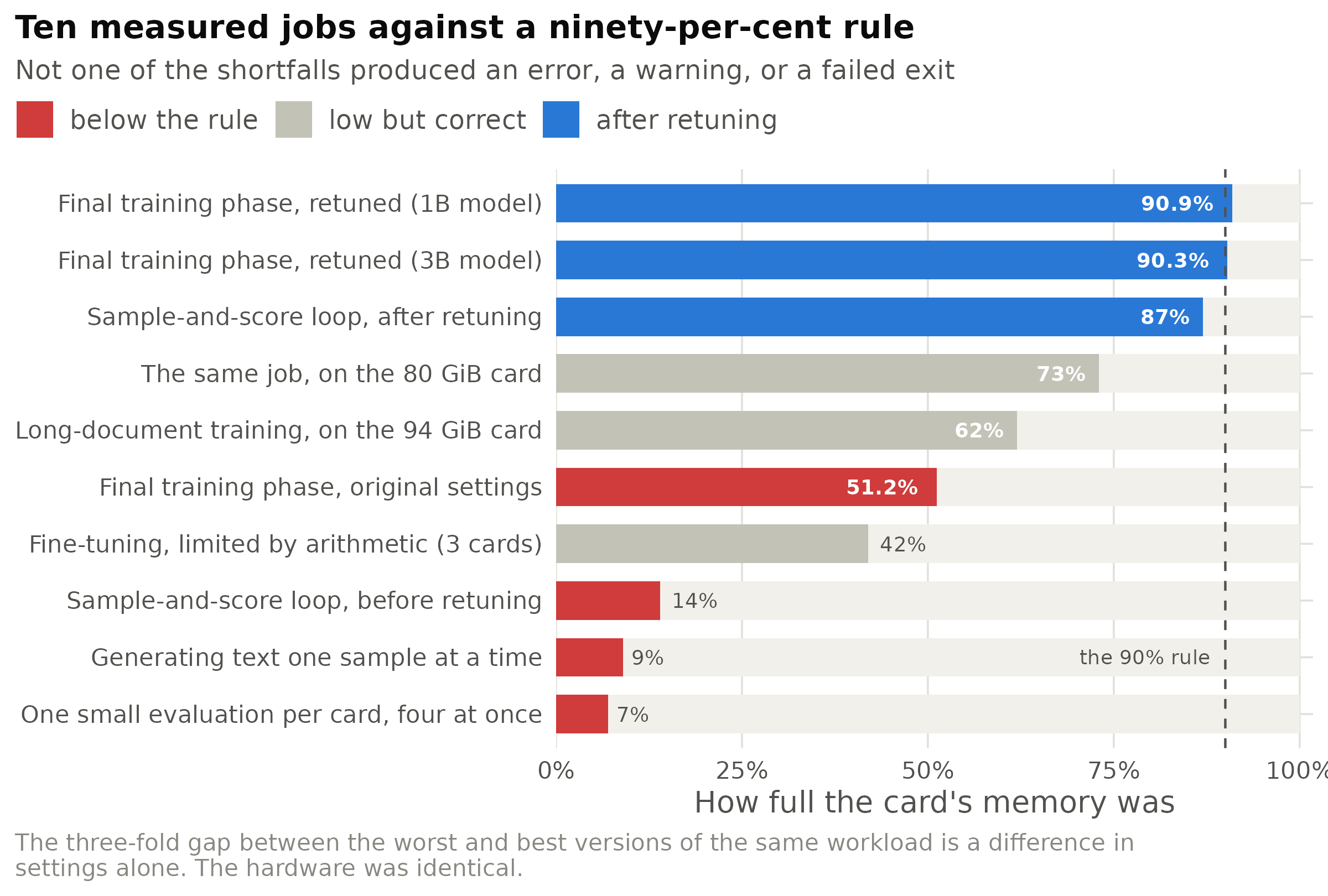
Figure 2: How full the graphics card was, across ten real jobs; the dashed line marks the ninety-per-cent rule and the faint bar behind each row is the whole card. Red is genuine waste: the same work would have fitted on a fraction of the card, or the same card could have done far more. Blue is the same workload after being reconfigured. Grey is the important complication — a low figure that is nonetheless correct, because the job was limited by arithmetic rather than by memory, or because it is quoted against a larger card than the one it may next land on.
None of these were failures in any sense the system recognises. Every job ran to completion and produced correct results. The text-generation job produced exactly the text it was asked for, at about forty words a second, on a card capable of ten to fifty times that. Nothing was logged, because from inside the program everything was fine.
And some of those low figures are right. The three-card fine-tuning job sat at forty-two per cent memory while keeping the cards ninety-nine to one hundred per cent busy: it was limited by arithmetic, not memory, and enlarging it to “fix” the figure would have broken comparability with the experiment it was reproducing. A tool that flags that job as unhealthy is worse than no tool, because it teaches its user to ignore it.
The fixes, once the numbers were known, were large and free. Four training stages were retuned on identical hardware.
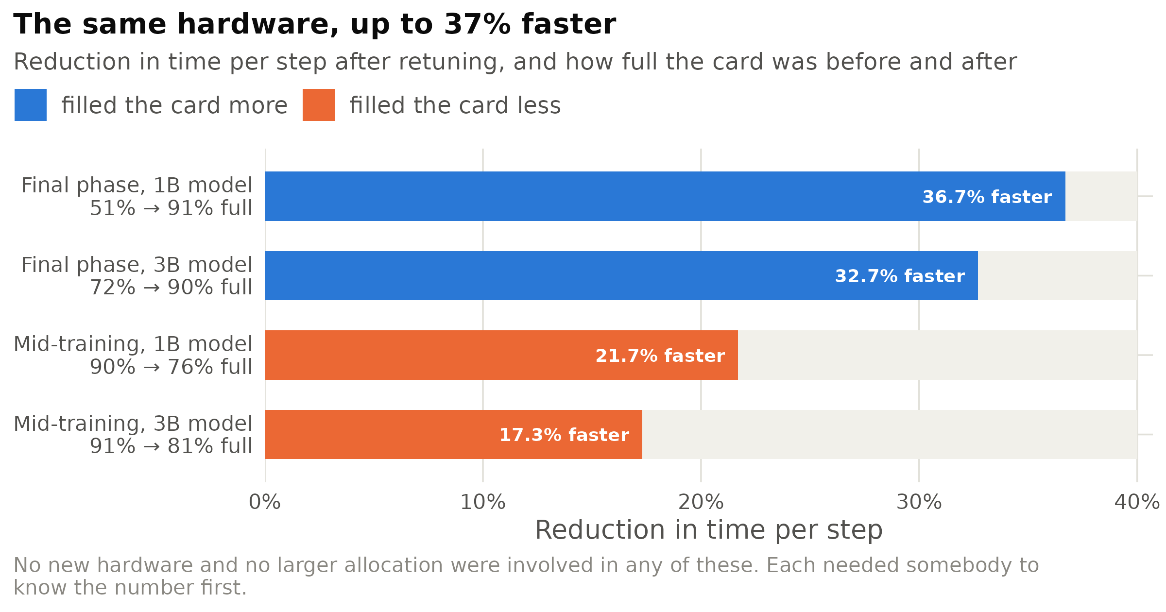
Figure 3: Time saved per step after retuning four training stages, on hardware that did not change. The label on each bar gives how full the card was before and after. Note the direction: two stages got faster by filling the card more, and two got faster by filling it less. Any rule that treats fullness as the target gets half of these backwards. On top of these, a fifth stage was verified in production at 403 steps per hour against 368 before — the same machine, the same hour, 9.6% more work.
That figure carries the article’s argument in one image. The gains are large, they cost nothing, and they run in both directions — so no fixed target for card fullness could have found them. Only measuring the time per step could.
The hundred-per-cent illusion
The most instructive failure in the record involved no shortfall at all. One fine-tuning job was run three ways, and its card reported one hundred per cent busy every time.
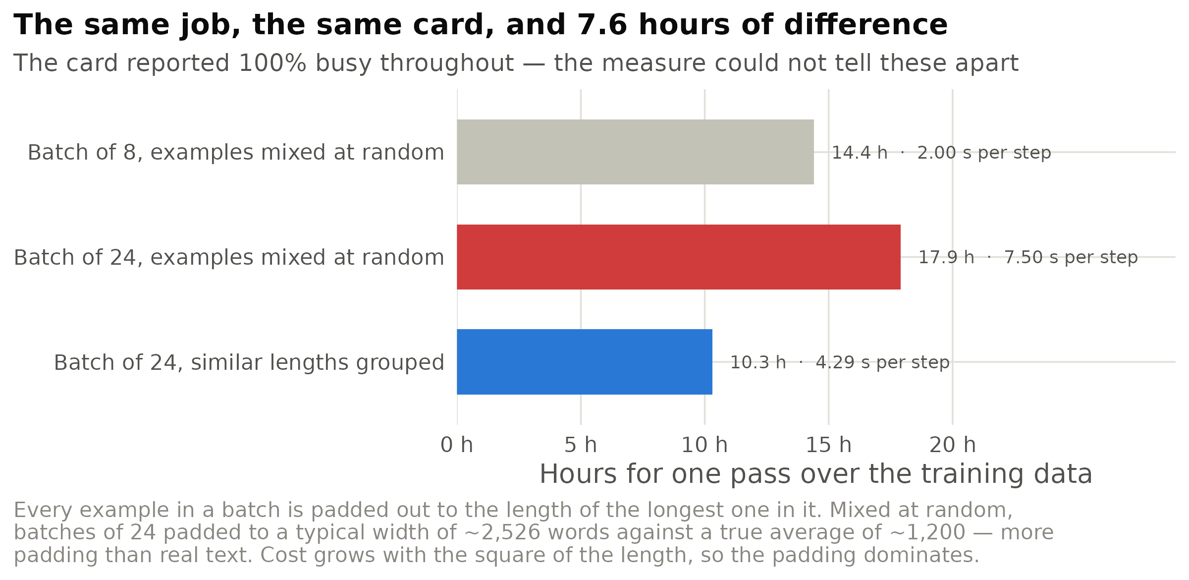
Figure 4: Hours to make one pass over the same training data, in three versions of one job on one card. Enlarging the batch to fill the card — the intuitive move, and the one the ninety-per-cent rule encourages — made the job 24% slower. Sorting similar-length examples into the same batch, so that far less padding is processed, then made it 1.74 times faster. The card reported 100% busy in both batch-24 versions.
The reason is padding. Examples in a batch must all be the same length, so every one is padded out to match the longest. Batches assembled at random padded to a typical width of about 2,526 words against a true average of about 1,200 — more padding than real text — and the cost of the underlying calculation grows with the square of the length. The card was genuinely one hundred per cent busy. It was one hundred per cent busy multiplying zeros.
This cuts against the tool this article introduces, and is worth saying plainly: neither the activity percentage nor the memory figure would have caught it. Only the time per step did. The activity figure reports the fraction of time during which the card had something to do, not how much work it finished. No instrument reports whether the work being done is work worth doing.
Filling the card is a means, not an end
The ninety-per-cent rule is a proxy, and the record shows cleanly where the proxy breaks down. The sweep below changes only how one internal calculation is broken into pieces, which alters how much memory is occupied without altering the result at all.
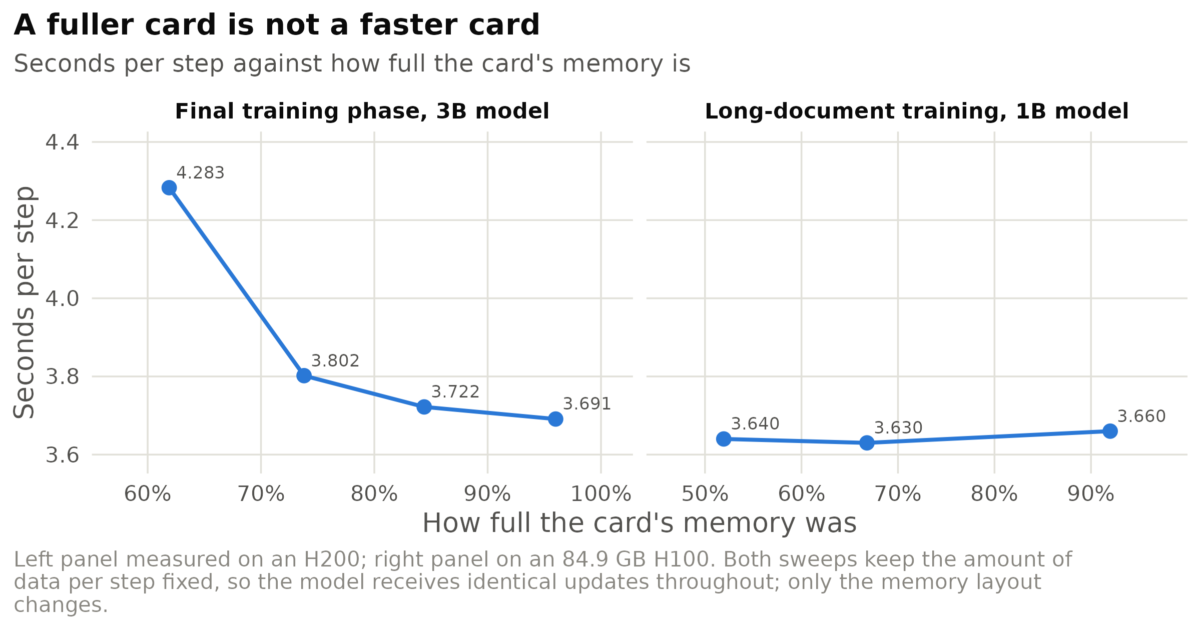
Figure 5: Step time against how full the card is, on two stages of the same project. The panels share a vertical axis, so the two shapes can be compared directly. Left: a real gain, but essentially exhausted by 84% — the last twelve percentage points of memory buy 0.8% of speed. Right: on long documents the line is flat, and an extra 34 GB of occupied memory buys nothing measurable. Elsewhere in the same record, settings that filled 96-99% of the card measured slower and less predictable than those at 84-93%.
The right target is therefore the fastest setting, which in this project consistently landed between eighty-five and ninety-three per cent, not at the ceiling. How full the card is remains worth measuring, because it is a strong hint — and worth measuring rather than predicting, because it is not a reliable one. The same record holds three memory predictions that failed in a single day, each made carefully and each caught only by going and looking. The lesson from all three is the same: do not extrapolate, measure.
A card at a fifth of its speed, and nothing in the log
The most expensive failure in the record was not a settings mistake at all. On two occasions, on two unrelated runs, a job landed on a machine whose card was electrically throttled — held back by its own protection circuitry.
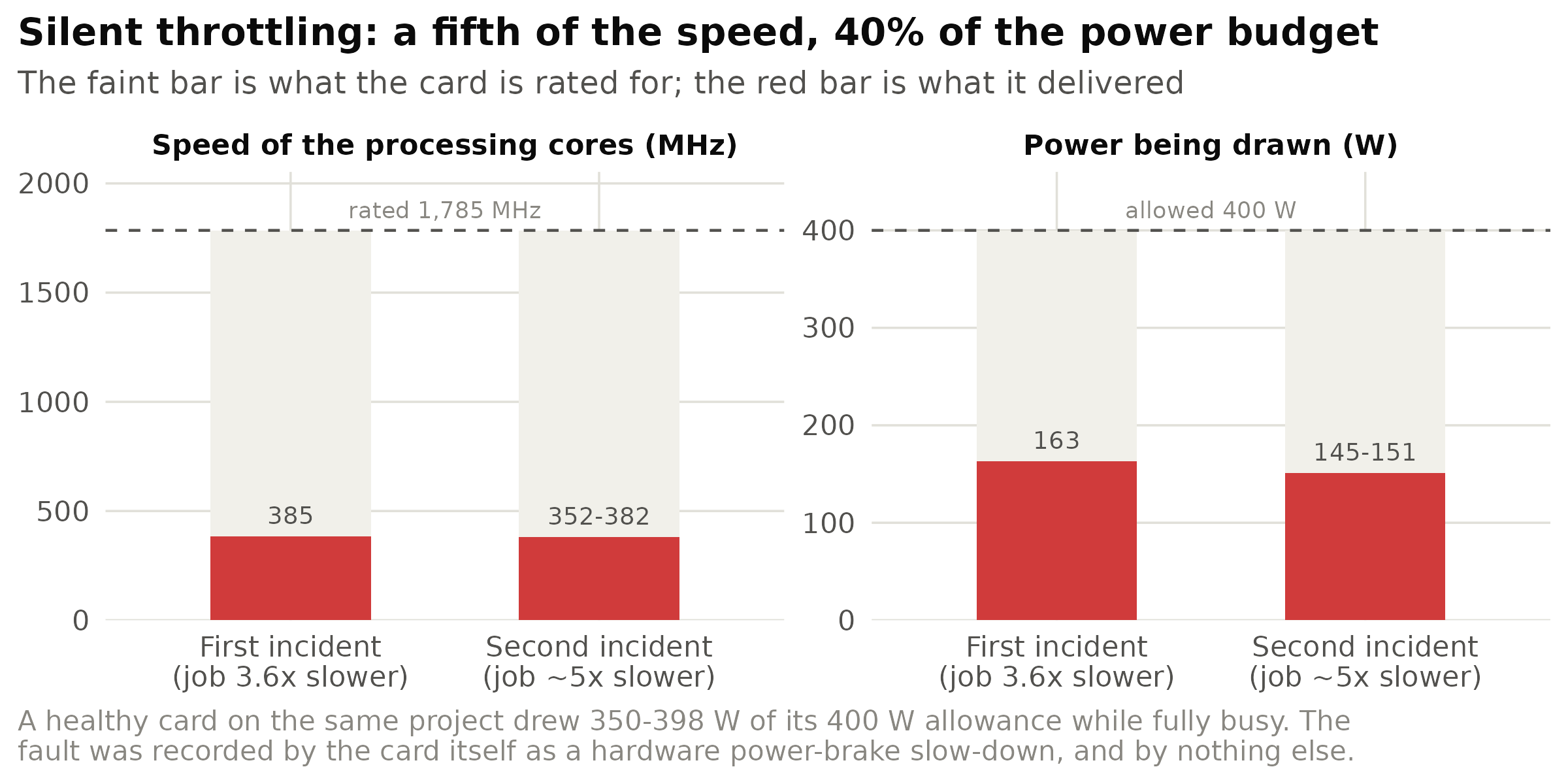
Figure 6: Two throttling incidents on the same machine, five weeks apart, on unrelated runs. The faint bar is what the card is rated for; the red bar is what it was actually doing. It ran at about a fifth of its rated speed while drawing roughly 40% of the power it was allowed, with a hardware slow-down flag raised the whole time. Red bars span the observed range where a range was recorded. Neither incident produced a single line in the job’s log.
In the first incident the card’s processing cores were pinned at roughly 385 MHz of a rated 1,785 — about twenty-one per cent — while it drew 163 W of a permitted 400 W at a cool 52 °C. The job ran three and a half times slower than it should have, and produced no error of any kind. Five weeks later the same fault recurred on the same machine and caught a different run: 352 to 382 MHz, 145 to 151 W, roughly a five-fold slowdown, noticed only because a monitoring loop happened to be reading the card’s speed.
This is the failure that most clearly demands readings taken on the machine itself. The program cannot detect it: every calculation returns the right answer. The scheduler cannot detect it: the job is running, where it was sent, within its time limit. A healthy card on the same project drew 350 to 398 W; a card drawing 163 W looks identical in every record the user can ordinarily see. The signal exists in exactly one place — the card’s own slow-down flag and its power draw against its limit — and somebody has to go and read it.
A job that looks broken and is not
Instruments cut the other way too. A resumed training job spends its first few minutes loading a large checkpoint from disk and compiling itself before it completes a single step. Throughout that window it looks exactly like a job that has hung.
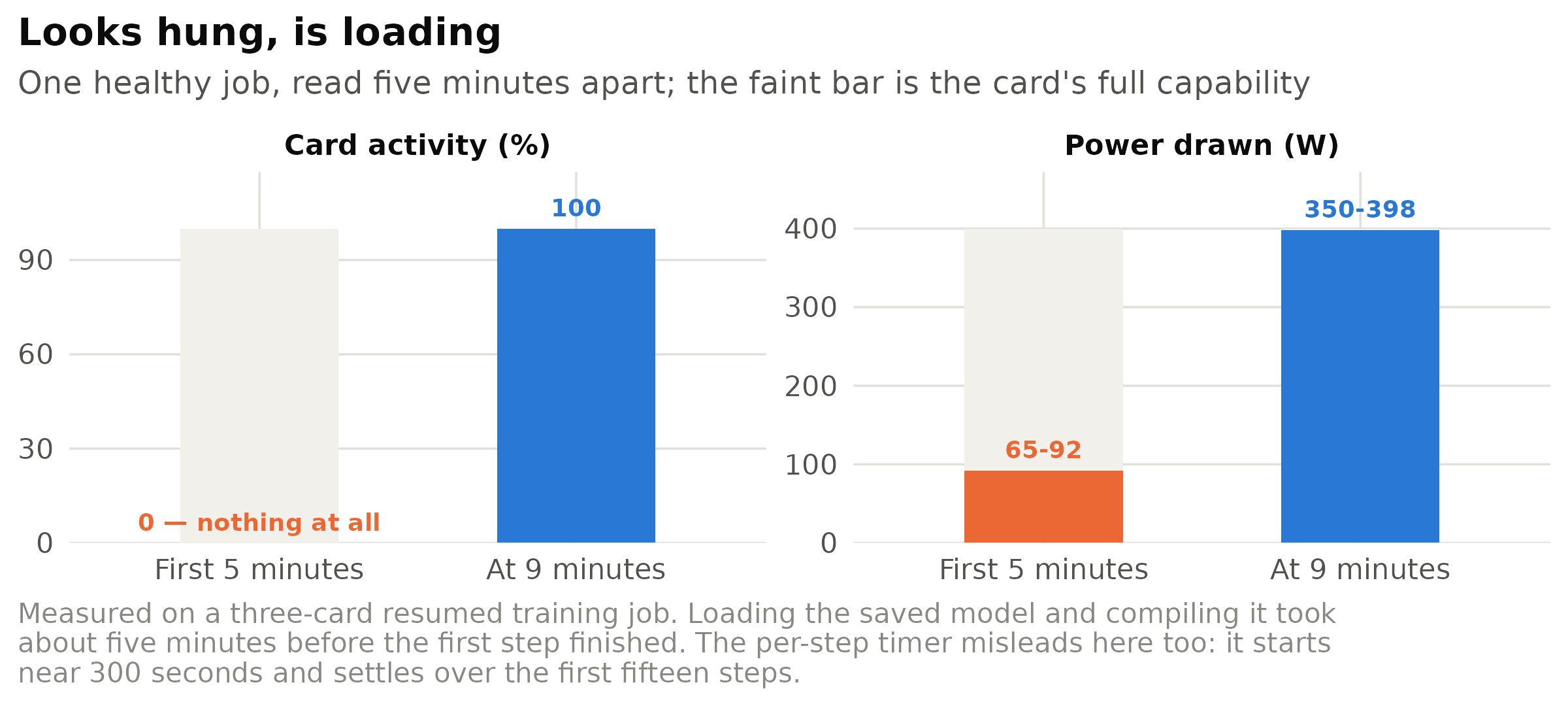
Figure 7: The same healthy job, measured twice. During the first five minutes it had reserved about 75% of the card’s memory while reporting no activity at all and drawing idle power — the classic signature of a job that has crashed and left its memory behind. Four minutes later it was fully busy at nearly its full power allowance. Bars span the observed range. The correct response to the left-hand reading is not a better instrument; it is a second reading, taken later.
This is the one failure in the record that node-local readings get wrong on their own. The lesson is not that the instrument is useless but that a single reading is a snapshot, and start-up is the one moment when the snapshot lies.
The same request, two different machines
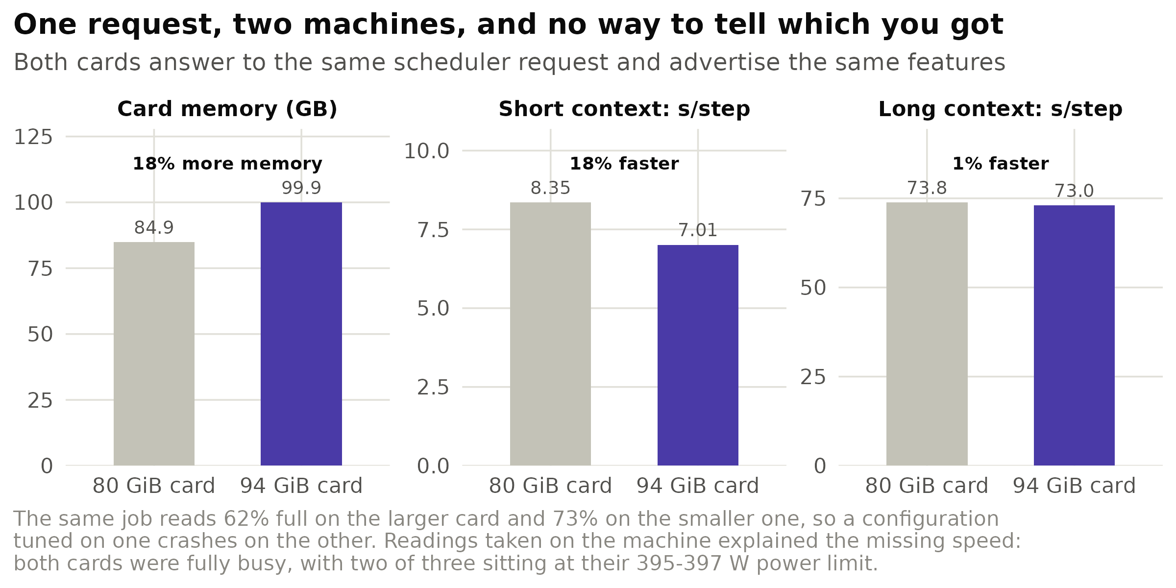
Figure 8: Two machines that answer to the same request. Asking the scheduler for an ‘H100’ returns either card; nothing distinguishes them, because they advertise themselves identically. The capacity gap is predictable. The speed gap is not: the larger card ran one job 18% faster and another job 1% faster. A time estimate built from the 18% figure predicted 63 seconds per step for the second job; it actually took 73.
The capacity difference is knowable in advance. The speed difference is not, and a prediction made from it was wrong by sixteen per cent. What settled it was reading the cards while the job ran: all were fully busy, and two of the three were sitting at their power limit — so the larger card’s usual advantage simply did not apply to this workload.
Which instrument sees which failure
Collecting all of the above, the matrix below summarises what each available signal reveals about each documented failure. It is deliberately unflattering to the tool this article introduces.
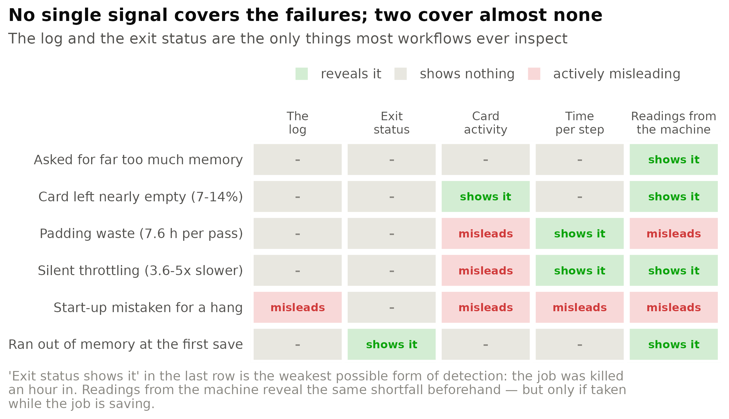
Figure 9: What each signal reveals about each documented failure. ‘Readings from the machine’ means how full the card is, power against its limit, slow-down flags, and the job’s true memory use — what slurmwatch reports. Two cells deserve comment. Card activity is marked misleading under throttling because that figure measures the fraction of time the card had something to do, not how much it finished, so a card at a fifth of its speed still reports fully busy. And the readings are marked misleading during start-up because the fix there is not a better reading but a second reading, taken a few minutes later.
Two columns deserve attention. The log — the one artefact that virtually every workflow, human or automated, actually inspects — reveals nothing about five of the six failures and misleads on the sixth. The exit status reveals one, by killing the job. Everything else required somebody to deliberately measure something on the machine.
Why this is still needed
It is fair to ask why any of this remains necessary. The jobs above were configured, launched, monitored, and debugged with the help of extremely capable AI systems. Those systems wrote the code, sized the requests, and read the logs. Why did they not simply notice?
The answer is not that the models were insufficiently intelligent. It is that the information was never in front of them. No amount of capability substitutes for a measurement nobody took.
Consider what an agent working on an HPC system can actually see: the script it wrote, the job’s printed output, and the queue. From those three things, every failure catalogued here is invisible. The over-requesting job’s log said nothing about memory at all. The padding-waste job’s log showed a falling loss and a plausible step time. The throttled job’s log showed a falling loss and a step time three and a half times too slow — but “too slow” means something only against a baseline, and on the first run of a new configuration there is no baseline. There is nothing here for a reader of any capability to notice, because the relevant fact was never written down.
This is structural, not a temporary limitation.
The failures are silent by construction. Nearly every incident here produced correct output and a successful exit. Software engineering’s entire apparatus for catching mistakes — exceptions, tests, type checkers, assertions — assumes a wrong program does something recognisably wrong. A job that computes the right answer while holding eleven times the memory it needs is not wrong in any way that apparatus can see. It is merely expensive.
Capability has outrun observability. A modern system will design a competent job in minutes. The bottleneck is no longer knowing what a good configuration looks like; it is finding out which one you are actually running — as the two indistinguishable cards above show, that is not something any amount of reasoning about the job can recover.
Prediction is not a substitute, and confident prediction is worse than none. Three careful memory predictions failed in a single day, and the estimate built on the “18% faster card” was wrong by sixteen per cent. Each was settled by a measurement that took minutes. An agent without instruments does not merely fail to notice such things — it reports, in good faith, that the job is running fine.
Automation raises the stakes rather than lowering them. A person launching one job a week may eventually notice it feels slow. An agent launching jobs continuously, unattended, overnight and across weekends will reproduce a silent misconfiguration hundreds of times before anyone looks. The second throttling incident was caught on a completely different run from the one being watched, purely because a monitoring loop happened to be reading the card’s speed. That is luck, not a system.
And somebody still has to exercise judgment. The forty-two-per-cent job was right. The
sixty-two-per-cent job was right. The fullest setting was slower than the middle one. The
hundred-per-cent activity reading was true and useless. A monitoring tool does not remove the need for
interpretation — it makes interpretation possible, by putting the numbers in front of whoever, or
whatever, is doing the interpreting. That is why the machine-readable output matters as much as the
dashboard: --once --json exists so an automated agent can hold the same facts a person would, while
they still matter rather than in a post-mortem.
The underlying principle is unglamorous and long predates machine learning. Systems become observable only when somebody builds the instrument. Compilers did not get fast because compiler authors got smarter; they got fast because profilers were written. The same relation holds here. An HPC system is expensive, heavily contended, and almost entirely opaque, and the one question that matters — is this job using what it was given? — is answered by nothing in the default workflow. Intelligence, artificial or otherwise, cannot reason its way to a number nobody measured.
Availability
slurmwatch is open source under the MIT licence.
- Package:
slurmwatchon PyPI —pip install slurmwatch(also installable withuv tool installorpipx). The current release is v1.1.0. - Source: github.com/PursuitOfDataScience/slurmwatch — including the tests, the automated checks, and the issue tracker.
It is written for Slurm systems and reads NVIDIA cards where they are present; contributions extending it to other schedulers and other hardware are welcome. It began as a tool I wrote for myself, because I had spent an embarrassing number of allocation-hours on jobs that were, in hindsight, obviously idle. The measurements in the second half of this article are the record of finding that out.