A Repeat-Rent Index From Rental Listings: External Validation and a Falsified Explanation for Its Level Bias
Contents 11 sections
Abstract. Official measures of rent inflation are accurate and slow. This article builds a unit-level repeat-rent index for the United States from 12.8 million rental listings, using the repeat-sales design of Bailey, Muth and Nourse (1963) with the variance correction of Case and Shiller (1987), and evaluates it against two external benchmarks. On timing the index validates: it turns before the leading commercial asking-rent index, it leads the consumer price index’s rent component by roughly eleven months, which is the lag that Adams, Loewenstein, Montag and Verbrugge (2024) attribute to the distinction between new and continuing tenants, and it orders metropolitan areas almost exactly as Zillow’s index does. On level it understates five-year cumulative growth by about ten percentage points. The article then tests the explanation that the data documentation itself proposes, namely that the sample is truncated by a rent filter. A dose-response design that re-estimates the index over twenty-five nested rent bands confirms the mechanism, estimates it at eighteen standard errors, and shows that it accounts for roughly one per cent of the discrepancy. A second candidate, the choice between opening and closing asking price, accounts for two per cent more. The residual is consistent with sample composition, which cannot be tested without an external unit-level benchmark. The methodological point generalises: a mechanism can be real, correctly signed and precisely estimated while being two orders of magnitude too small to matter.
1. Introduction
Housing is the largest single expense in most household budgets, and the rent survey behind the consumer price index drives roughly a third of that index’s total weight: 7.6 % through rent of primary residence directly, and a further 26.6 % through owners’ equivalent rent, which the Bureau of Labor Statistics estimates from the rents of comparable rental units (BLS 2026a). Yet that survey is deliberately slow. It samples what tenants actually pay, including the large majority who are in the middle of a lease and whose rent will not change this month. That is the correct object for a cost-of-living index and the wrong object for anyone who needs to know what the rental market is doing now.
Online listings offer the opposite trade-off, and the case for using them is by now well established in price measurement generally: posted online prices are timely, enormous in volume, and free of the response burden of a survey, at the cost of measuring something slightly different from the transaction (Cavallo and Rigobon 2016). An advertised rent is visible the day it is posted, but it is an asking price: no lease has been signed, no tenant is observed, and the set of units advertised is whatever the platform happens to index.
The specific question here is whether a listings-based rent index can be made to behave: whether it tracks the established series, whether it leads them, and (the part that usually goes unexamined) whether the ways in which it fails can be diagnosed rather than merely disclosed. The answer is split, and the split is the contribution. The index validates on timing and fails on level, and the leading published explanation for that failure turns out, on testing, to be almost entirely wrong.
Three literatures meet here. The repeat-sales design originates with Bailey, Muth and Nourse (1963) and acquired its standard variance correction in Case and Shiller (1987, 1989). Its application to rents rather than sale prices is due to Ambrose, Coulson and Yoshida (2015), who introduced the repeat rent index and showed that rent indices built this way differ from the BLS series for reasons of sampling and construction; the same authors later traced the consequences for measured inflation (Ambrose, Coulson and Yoshida 2023). The asking-versus-contract-rent distinction, which governs every comparison in Section 4, was quantified using CPI microdata by Adams, Loewenstein, Montag and Verbrugge (2024). And the selection problem that Section 8 ends on (that units observed twice are not a random sample of the stock) was formalised for repeat-sales indices by Gatzlaff and Haurin (1997).
2. Data
The source is a corpus of United States rental listings supplied by Dwellsy and acquired by the University of Chicago Booth School of Business Center for Applied Artificial Intelligence (CAAI 2026): 12,796,708 de-duplicated listings from 2020 to 2026, a separate log of 24.3 million timestamped rent revisions, and a 101-week panel. Three properties of it govern everything below.
These are asking prices. No lease is signed and no tenant is observed. Coverage is whatever Dwellsy indexes, which is not a probability sample of the housing stock.
The listing is the wrong unit of analysis. Dwellsy expires listings automatically after 120 days, which splits one marketing episode for one apartment into several listing records. Measuring rent growth across listing records therefore mixes genuine price change with an administrative rule. The remedy is to work at the level of the unit (a specific apartment at a specific address) and to compare a unit only with itself.
The rents are filtered, not clipped. Dwellsy retains listings between $500 and $20,000 per month. Listings outside that range are absent from the data rather than winsorized to the boundary, so the number that were dropped is unknowable from the file. Sections 6 and 7 are about this property.
3. Estimator
3.1 Holding the apartment fixed
The design is the repeat-sales regression of Bailey, Muth and Nourse (1963), transplanted from house prices to rents as in Ambrose, Coulson and Yoshida (2015). Rather than compare the average rent this month against the average rent last month, which moves whenever the mix of advertised units changes, it uses only apartments observed twice, and asks how much the rent on that same apartment changed between the two dates. Every fixed characteristic of the unit, observed or not, differences out. A national index is then the set of monthly values that best reconciles all such pairs at once.
Matching is deliberately strict: consecutive listings at the same address identifier, the same bedroom count, floor area within five per cent, and a discarded tail of implausible changes. That yields 5,775,959 matched pairs with a median gap of five months.
3.2 Weighting and identification
Pairs are not equally informative. The longer a unit sits between two listings, the further its rent can drift from the market for reasons peculiar to that unit, so treating a fifty-month pair as though it were as precise as a one-month pair over-weights exactly the noisiest observations. Case and Shiller (1987) correct for this by modelling the residual variance as a function of the interval and re-estimating by generalised least squares. Their three-stage procedure is what the index below uses, and the first stage of it is visible directly in the data.
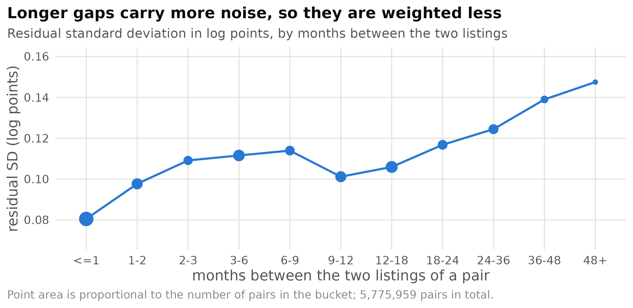
Figure 1: Standard deviation of the repeat-sales residual by the gap between the two listings of a pair. The generalised least squares stage weights each pair by the inverse of this fitted variance. The dip at nine to twelve months is the annual lease cycle: pairs almost exactly a year apart are unusually well behaved.
The second requirement is that a repeat-sales index is only identified in months that actually contain pairs.
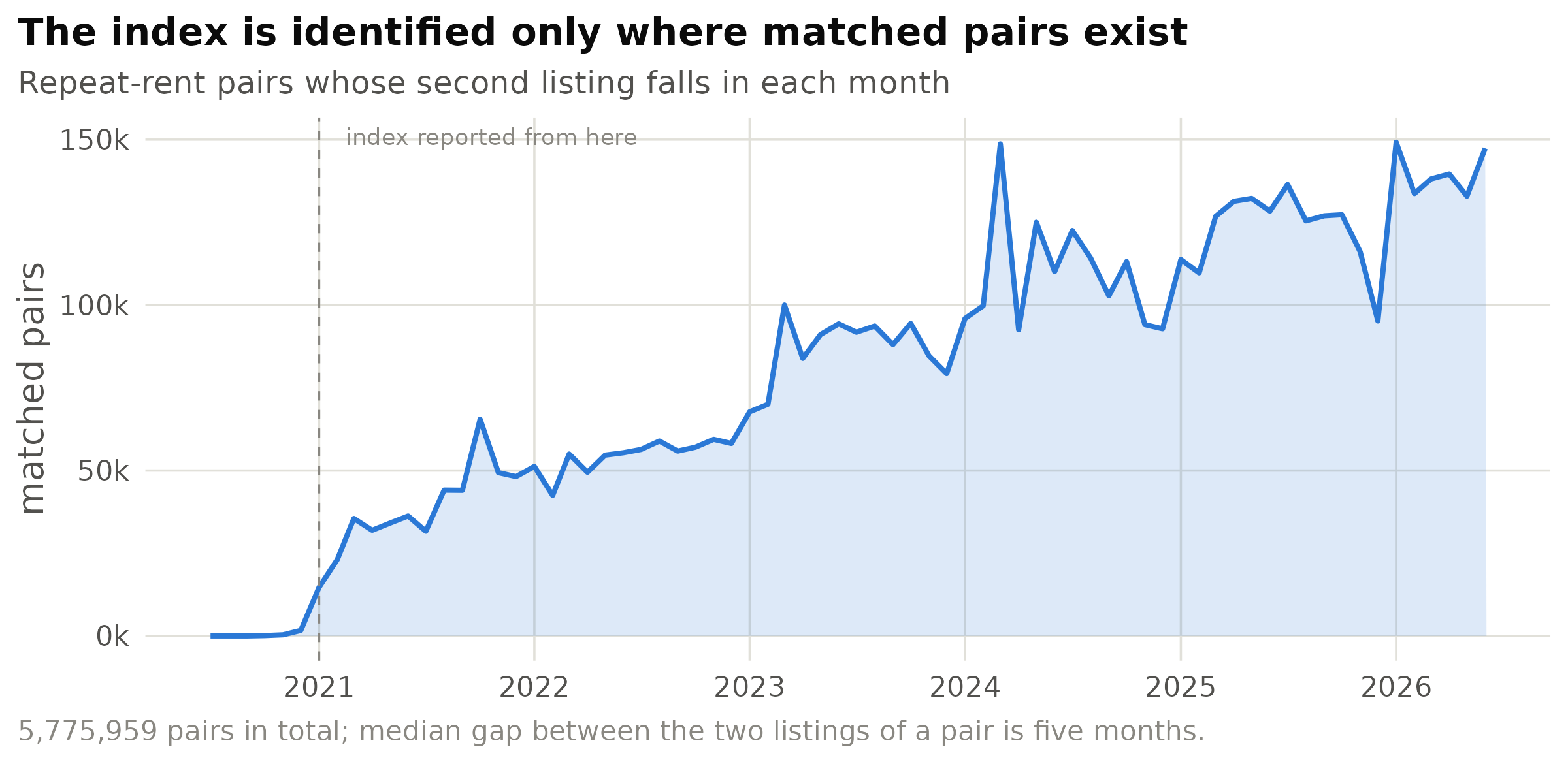
Figure 2: A pair is dated by its second listing, so the count is mechanically zero at the start of the window and thin for the first half-year; the index is reported from 2021-01 for that reason. The upward drift thereafter is the panel accumulating history, not a rising re-listing rate.
4. External validation
The comparison series are Zillow’s ZORI, itself a repeat-listing asking-rent measure but one that reweights to the rental housing stock using census benchmarks (Zillow 2026), and the CPI’s rent of primary residence, which is contract rent paid by sitting tenants. The prediction stated before looking was that ZORI should track closely and the CPI should not, and specifically that agreement with the CPI at zero lag would be evidence of a problem rather than of success, because the two series measure different things at different points in a tenancy (Adams et al. 2024).
4.1 Levels and turning points
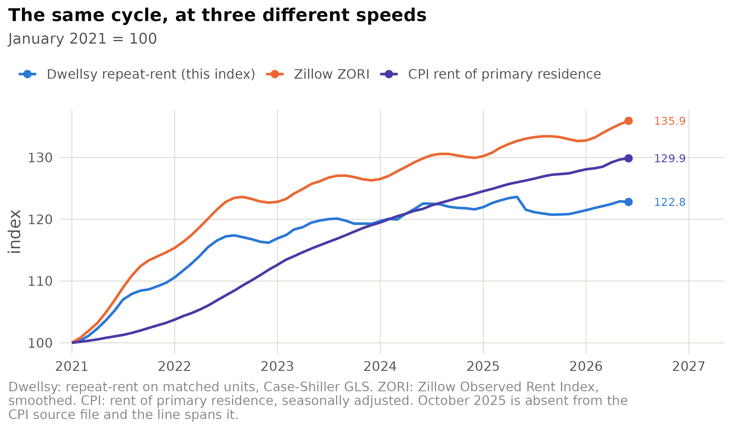
Figure 3: All three series are indexed to 100 in January 2021. The Dwellsy index reaches its peak and turns over well before either comparison series does; the CPI, which is contract rent paid by all tenants rather than the rent asked of new ones, is still climbing when asking rents have been flat for a year.
The shapes agree and the timing does not, which is the intended result. Correlation in levels is uninformative here because all three series trend upward; the demanding test is the correlation of month-to-month changes, and the informative statistic is the lag at which that correlation is maximised.
4.2 The lead over contract rents
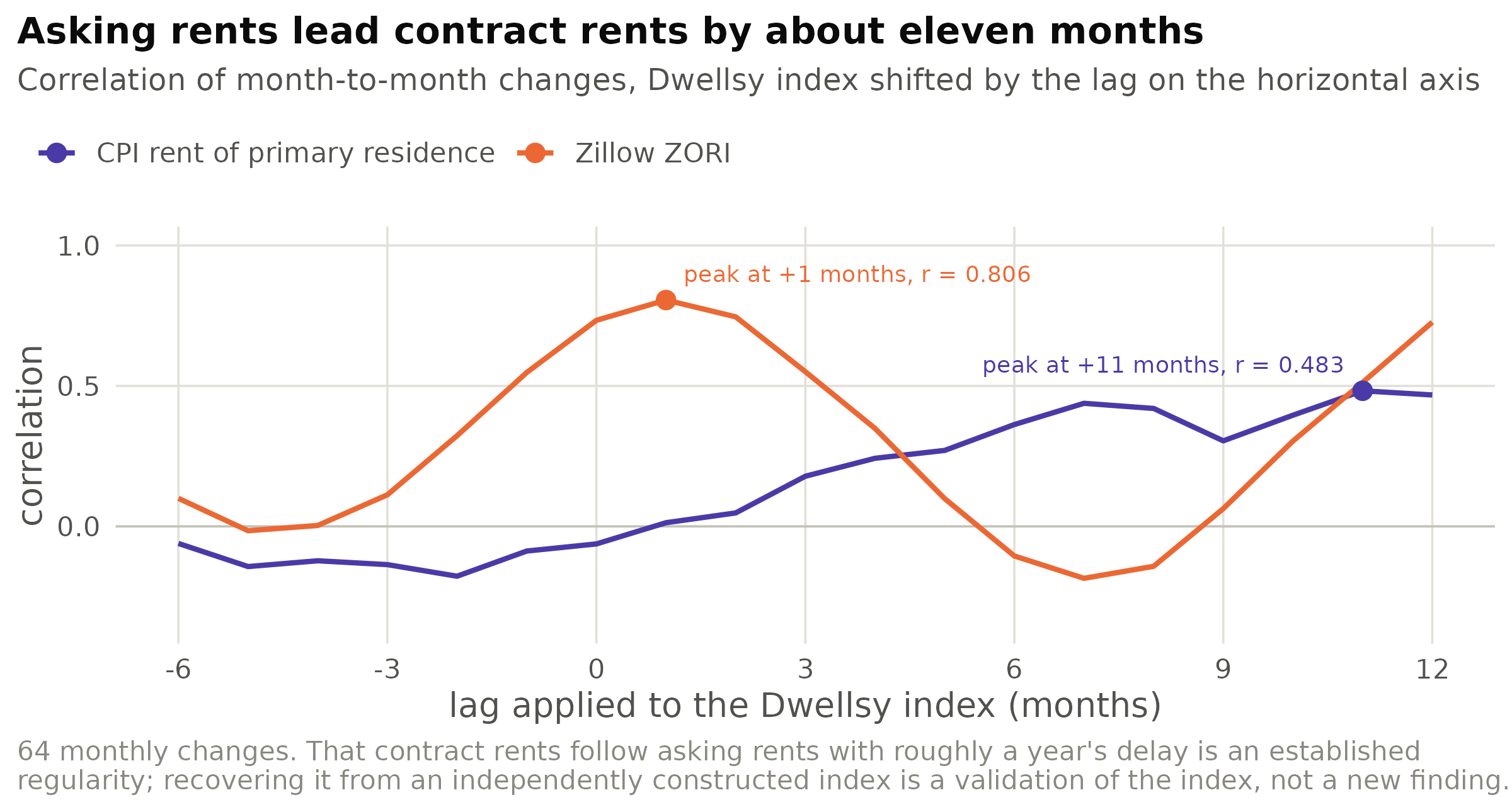
Figure 4: Cross-correlation of month-to-month changes at each lag. A positive lag means the Dwellsy index moves first. Against ZORI the peak sits at one month, the offset expected from ZORI’s own smoothing. Against the CPI it sits at eleven months, and the contemporaneous correlation is approximately zero.
This lag is not a discovery, and that is exactly why it is useful. Adams et al. (2024) show, using the CPI’s own microdata, that the reason alternative rent indices diverge from CPI shelter is that they measure rent inflation for new tenants while the CPI measures it for all tenants, and that new-tenant rent inflation therefore forecasts the official series. The Bureau of Labor Statistics now publishes a New Tenant Rent Index on precisely this logic, which secondary analyses place roughly six to twelve months ahead of CPI rent (BLS 2026b). Recovering an eleven-month lead from an index built on different data by a different method is corroboration that the index measures what it claims to.
4.3 The metropolitan cross-section
Restricting to metropolitan areas with at least 25,000 matched pairs and joining to ZORI gives 46 metros.
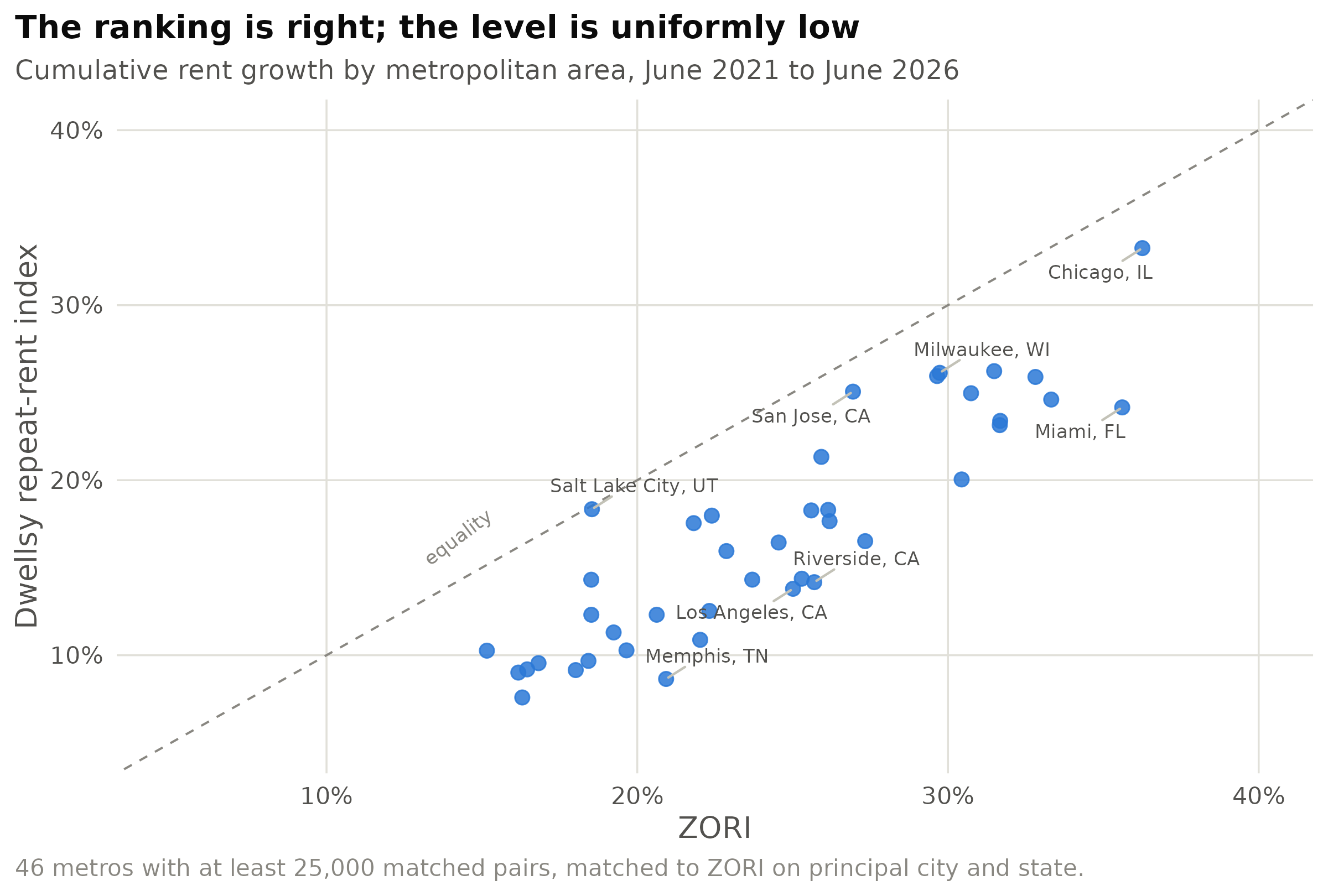
Figure 5: Each point is a metropolitan area; the diagonal is equality. The rank correlation is 0.92, so the index orders metros almost exactly as ZORI does, but every one of the 46 points lies below the diagonal, which is a systematic level difference and not scatter.
4.4 Beyond the 46 metros
Metropolitan areas are defined on core-based statistical areas, so a metro-only view leaves most of the map blank and says nothing about small-town or rural rental markets. The same matched pairs support a state-level index directly (every state clears five thousand pairs), estimated with the identical procedure used nationally.
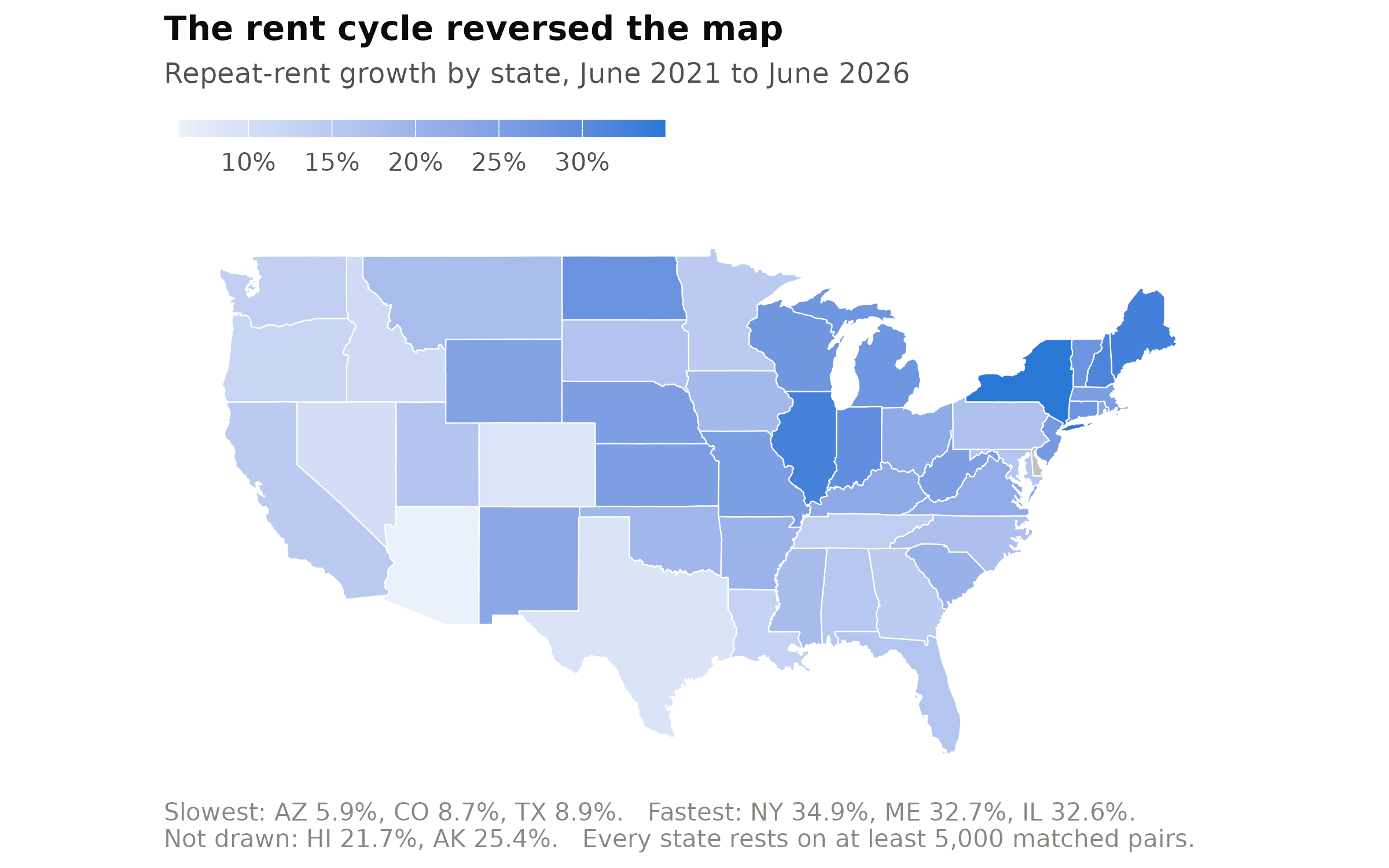
Figure 6: Cumulative growth June 2021 to June 2026, estimated separately for each state on the same matched pairs and the same estimator as the national index. Alaska and Hawaii are estimated and labelled below but are not drawn, as the base map is the lower 48.
The states that led the pandemic-era surge are the states that gave it back. This is the spatial signature that Gupta, Mittal, Peeters and Van Nieuwerburgh (2022) identified in the pandemic revaluation of urban real estate, now observed in reverse: the bid-rent curve that flattened in 2020 and 2021 has been steepening as the largest multifamily construction wave since the mid-1980s delivered into exactly the Sun Belt markets that had run hardest (CBRE 2025).
County resolution requires a different estimator. A repeat-sales index needs pairs in enough separate months to chain, and the typical county has a few hundred pairs spread over five years. What is identified at that resolution is the duration-weighted mean within-unit growth rate: total log rent change across all matched pairs in the county, divided by the total elapsed time those pairs span. It uses the same pairs and the same unit test, and it is a period-average annual rate rather than a chained index, so it should not be read against the state numbers digit for digit.
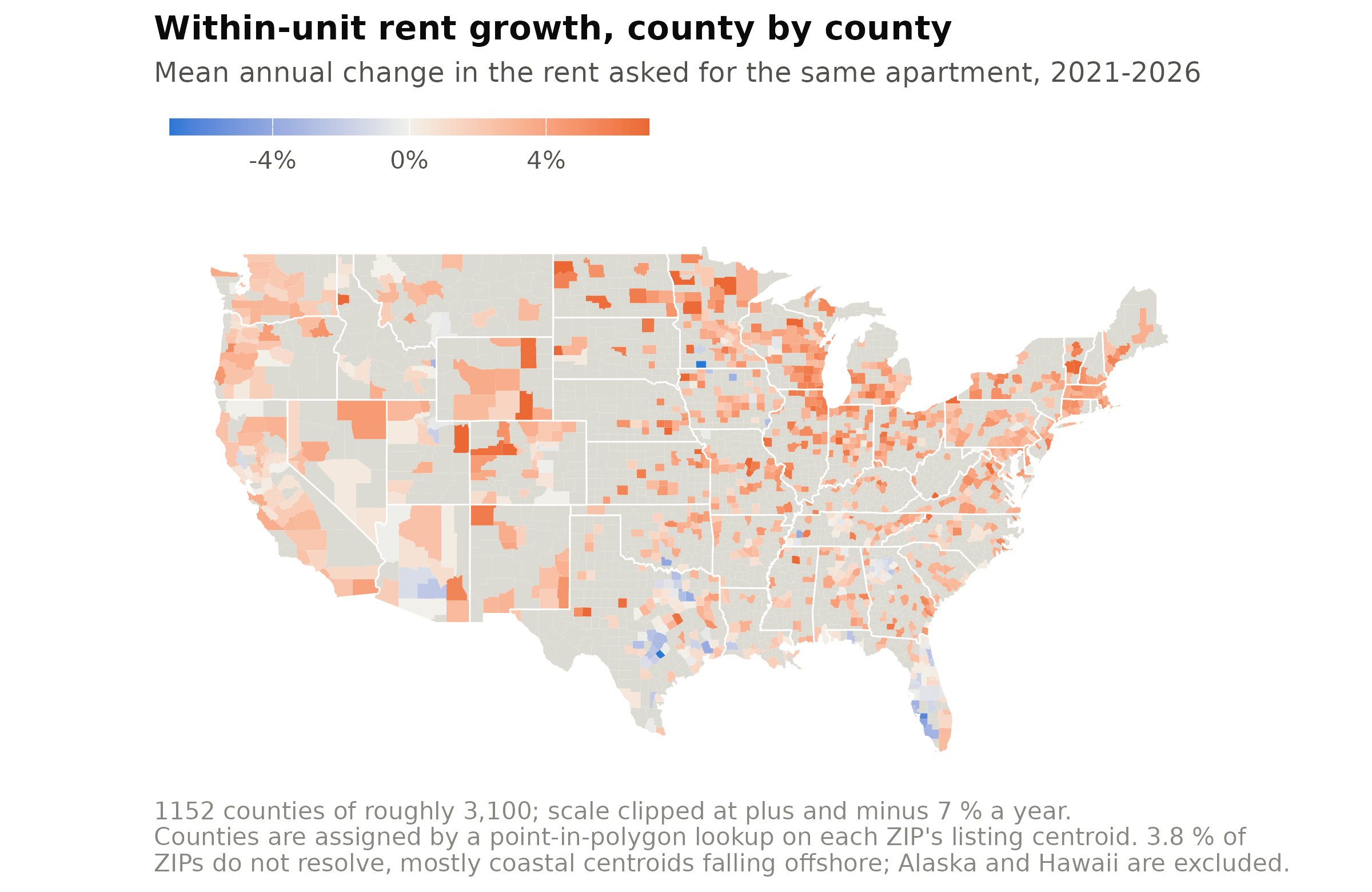
Figure 7: Duration-weighted mean within-unit rent growth per year, 2021 to 2026, for the 1,152 counties with at least 100 matched pairs. Counties in grey have too few pairs or no listings at all. Rents are measured on the same apartment twice, so none of the variation here is composition between counties.
5. The level discrepancy
Every point in the metropolitan cross-section sits below the diagonal, and the national series does the same thing: the index reproduces the shape and the timing of the rent cycle while understating its size. The natural first suspicion is that this is an artefact of holding the unit fixed, since a repeat-rent design deliberately discards everything except units that appear twice, the concern Gatzlaff and Haurin (1997) raise. It is not.
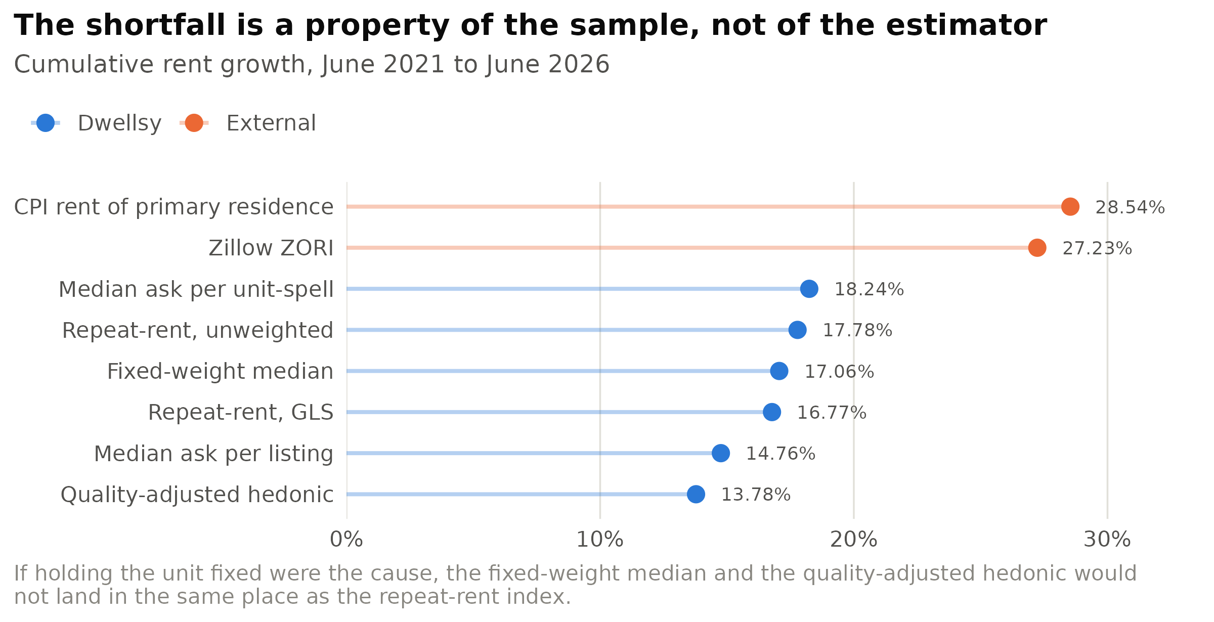
Figure 8: Six ways of measuring the same quantity on the same data, against the two external series. The Dwellsy estimators differ in almost every respect (one holds the unit fixed, one holds the composition fixed, one adjusts for observable quality), and they agree with each other far more closely than any of them agrees with ZORI or the CPI.
A repeat-rent index, a fixed-weight median and a quality-adjusted hedonic regression are three different answers to three different questions, and they disagree with one another by about four percentage points. All six land below nineteen per cent while both external series land above twenty-seven. Whatever produces the gap therefore sits upstream of the estimator, in which listings are present in the sample at all.
Two candidate mechanisms are testable inside the data. Sections 6 and 7 test them.
6. Hypothesis 1: the rent filter
6.1 Mechanism
The $500 to $20,000 bound is a row filter: out-of-range listings were never written to the file. In a repeat-rent design that has a specific and unpleasant consequence, because a pair survives only if both of its listings fall inside the band. Consider an apartment advertised at $470 in 2021 and at $560 in 2023. It rose by nineteen per cent, and it contributes nothing to the index, because its first listing was never recorded. The apartment next door, advertised at $520 and then $560, rose by eight per cent and does contribute. At the lower edge of a rising market the filter preferentially deletes the units that rose the most, and the same argument at the upper edge deletes units that rose out of the top of the band.
The prediction that follows is sharp enough to be wrong: attenuation must be dose-dependent. Narrowing the band should attenuate the measured index further, from each side independently, and monotonically in how much of the market the band excludes.
6.2 How large is the dose?
Before testing the prediction, the size of the dose has to be estimated, and this is the part that cannot be done from the data alone: the mass outside the band is unobservable by construction. What can be done is to fit a distribution to a region of the observed data that is safely interior (far from both boundaries, so no boundary distortion enters the fit), and extrapolate it outward. Fitting a lognormal to observed rents between $1,000 and $8,000 by maximum likelihood, with the truncation of the fitting window itself entering the likelihood, gives the following picture.
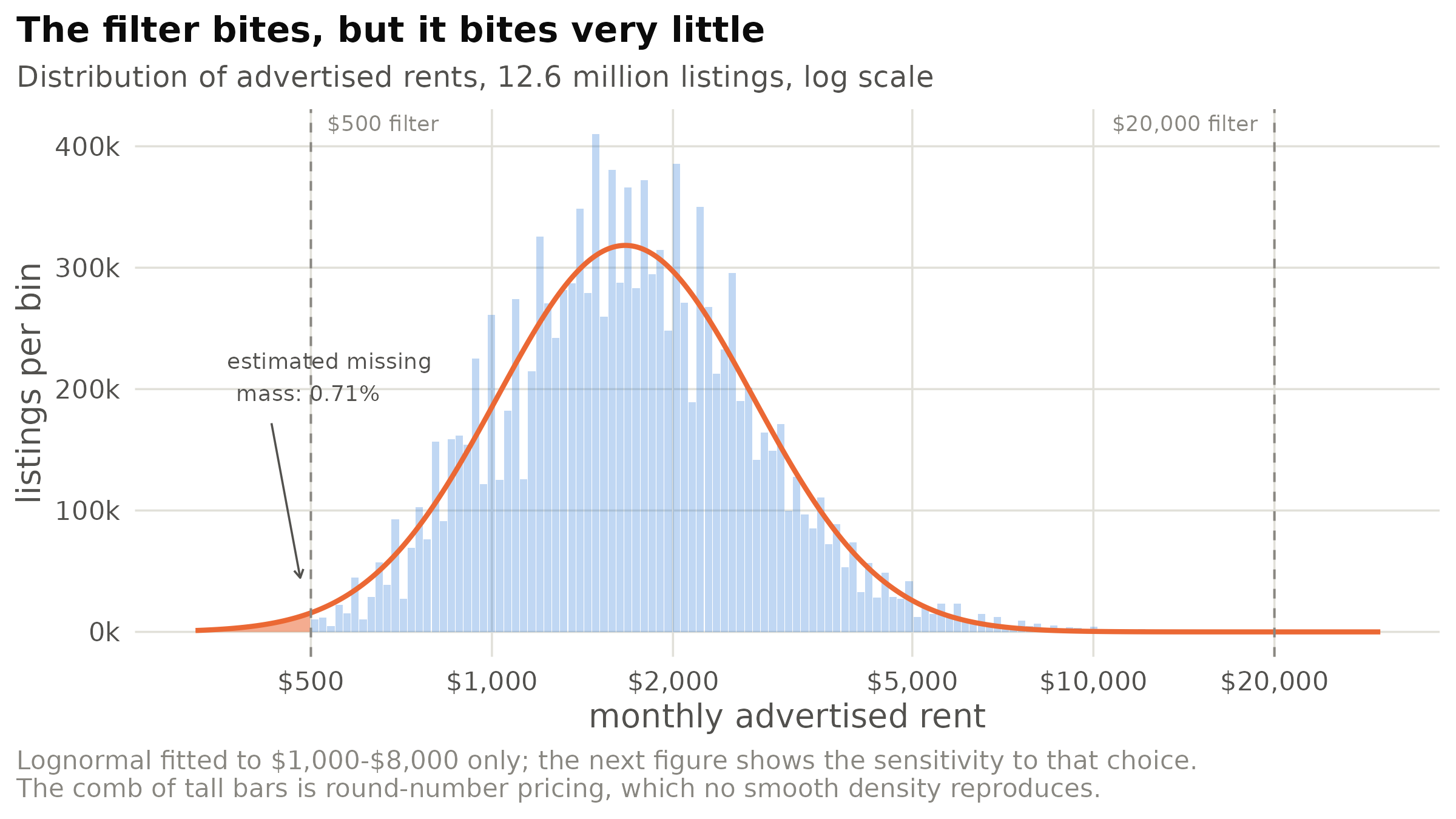
Figure 9: Observed advertised rents (bars) with a lognormal fitted by maximum likelihood to the interior region between $1,000 and $8,000 (line), extrapolated past both boundaries. The shaded area below $500 is the estimated missing mass. The upper bound is far into the tail and removes essentially nothing.
The median advertised rent is $1,679 and the fifth percentile is $795, so the lower bound sits deep in the left tail and the upper bound is effectively irrelevant: one listing in seven thousand is within ten per cent of it. How much the filter removed depends on the fitting window, and on the year: as the rent distribution shifted right over the window, it pulled away from the lower bound and the filter bit progressively less.
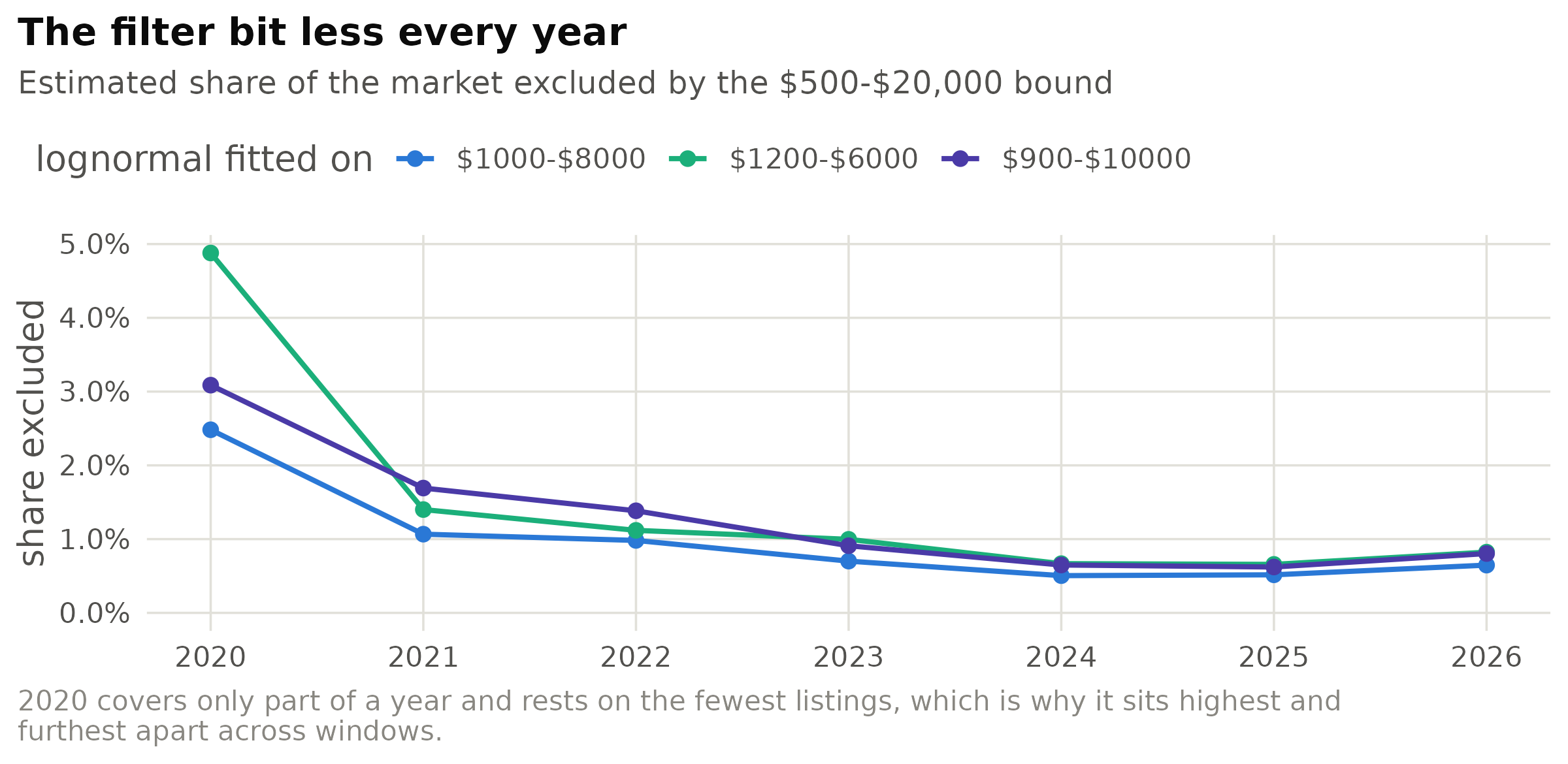
Figure 10: Estimated share of the underlying rent distribution falling outside the $500-$20,000 band, fitted separately for each year and each of three interior windows. The spread between the three lines is the model uncertainty on a quantity that cannot be observed; the downward slope is the distribution shifting right, away from the lower bound.
6.3 The dose-response test
The index was re-estimated on progressively narrower bands: from both sides at once, from the bottom only, and from the top only. Everything else (the pair construction, the unit test, the trim, the Case-Shiller weighting) is held identical, so the only thing that varies between points is how much of the market the band admits.
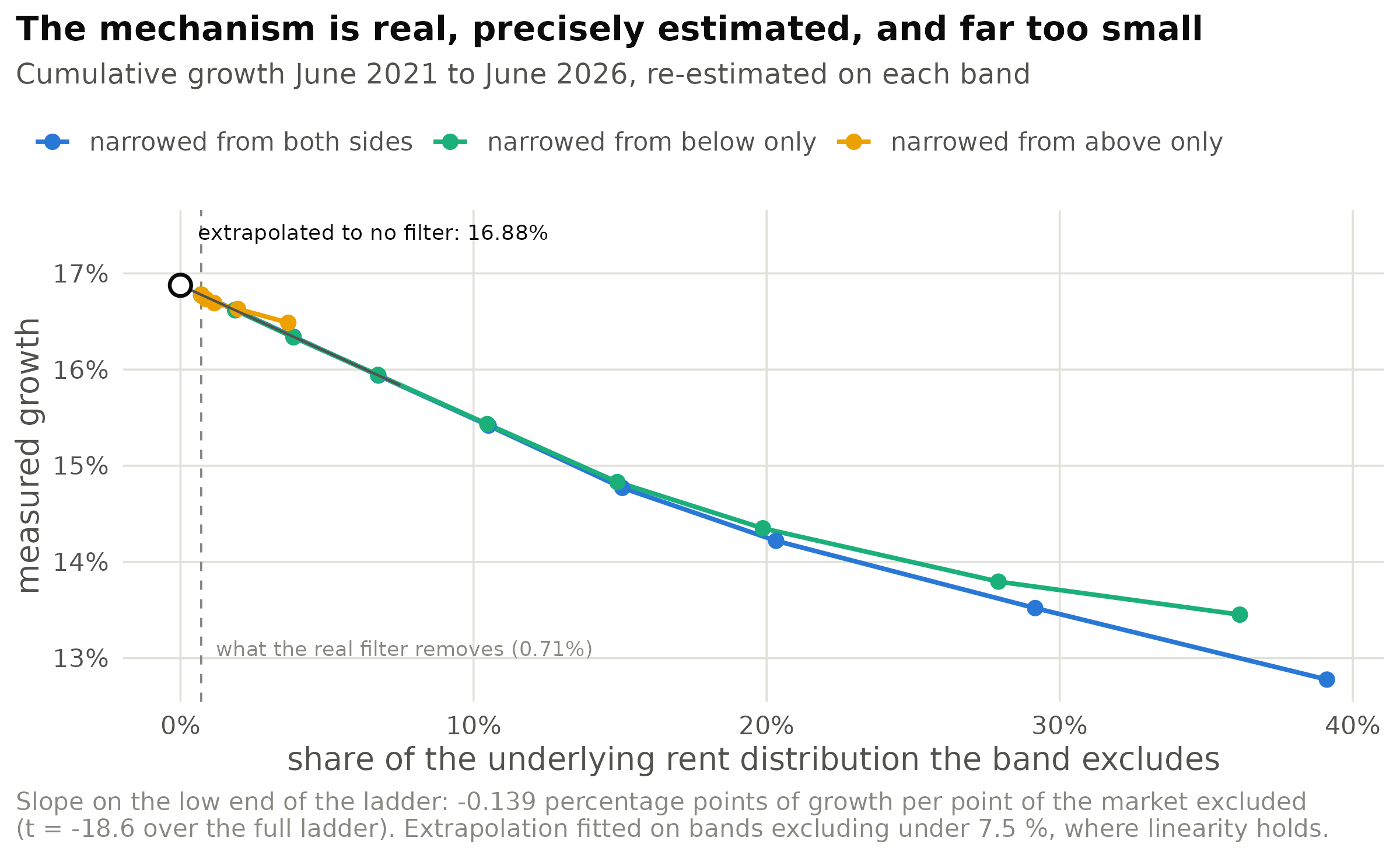
Figure 11: Each point is a complete re-estimation of the national index on a narrower band. The mechanism is confirmed: growth falls monotonically as the band excludes more of the market, from both directions, and the slope is estimated precisely. The extrapolation to an unfiltered sample is the open point at the left.
The prediction holds in every respect. Growth falls monotonically as the band tightens; it falls when the band is tightened from below and, much more weakly, when tightened from above, which is what the shape of the distribution implies it should do; and the relationship is close to linear over the region that matters. Discarding two-fifths of the market costs four percentage points of measured growth, so the mechanism is not merely present but large when the dose is large.
6.4 Verdict
The dose, however, is not large. Removing the estimated share that the real filter removes moves the index by about a tenth of a percentage point.
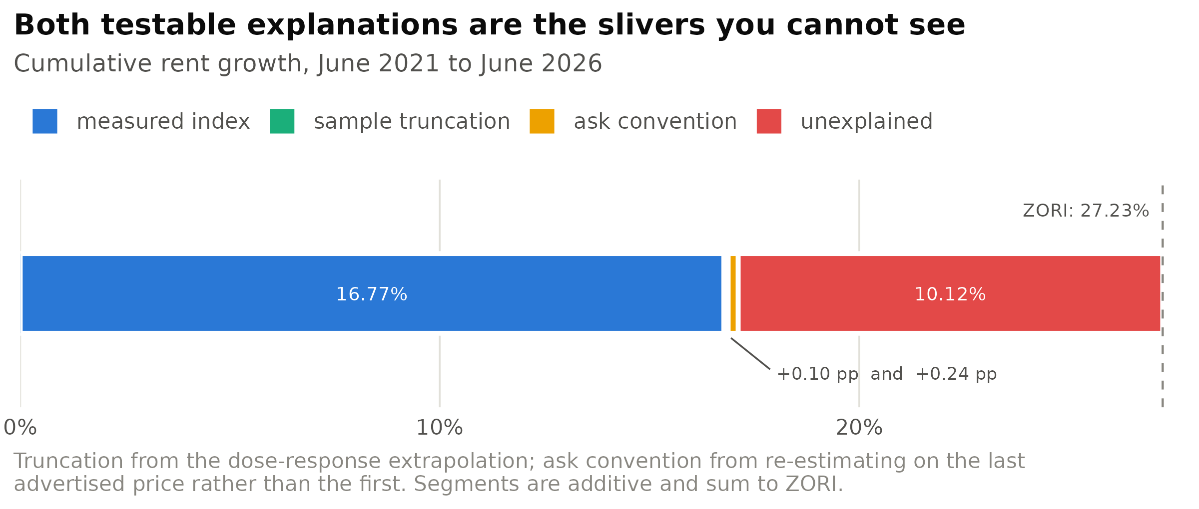
Figure 12: Decomposition of the ten-and-a-half point discrepancy against ZORI. Both mechanical explanations are real and both are negligible; the residual is not a rounding difference but the overwhelming majority of the gap.
7. Hypothesis 2: which asking price is indexed
Every listing has at least two prices: the one it opened at, and the one it carried when it left the market. The index above uses opening asks. If landlords increasingly marked down while a unit sat, an opening-ask index would miss a growing discount.
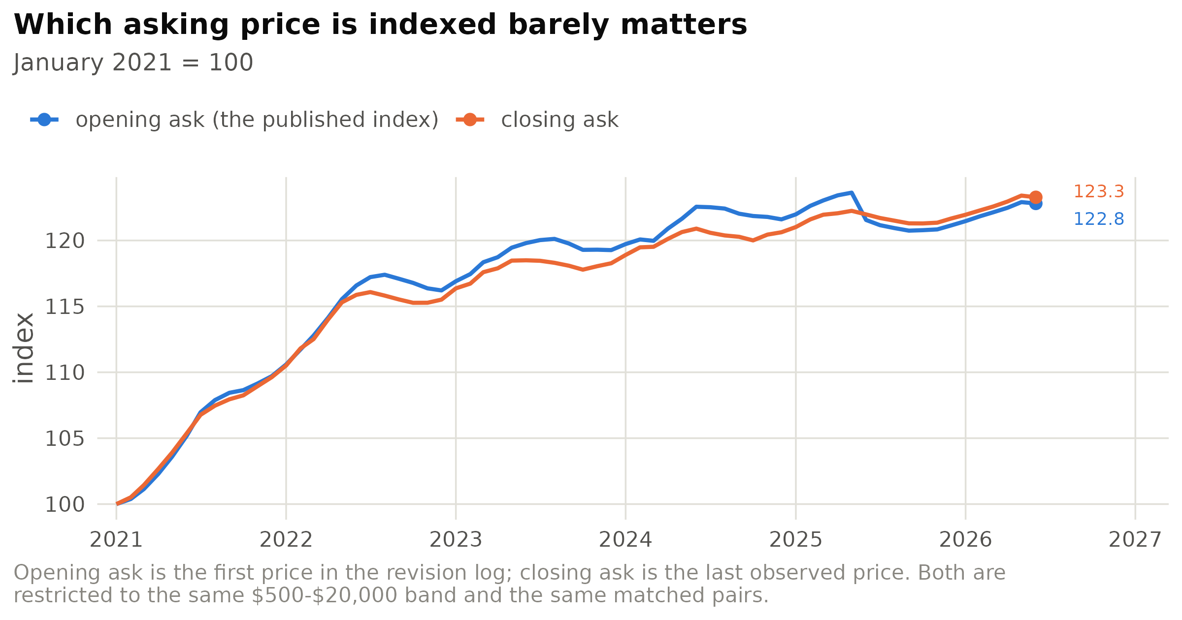
Figure 13: The same estimator, the same units and the same band, run once on the price each listing opened at and once on the price it carried when it left the market. The two paths are almost indistinguishable, and the five-year totals differ by roughly a fifth of a percentage point.
That the substitution changes so little is worth a moment, because the two prices are not close to interchangeable at the level of the individual apartment. A separate decomposition on the weekly panel separates the two decisions a landlord makes: the re-listing step, which is the new asking price relative to the last asking price of the previous listing at the same unit, and the within-spell markdown, which is how far the price is walked down while the unit sits unrented.
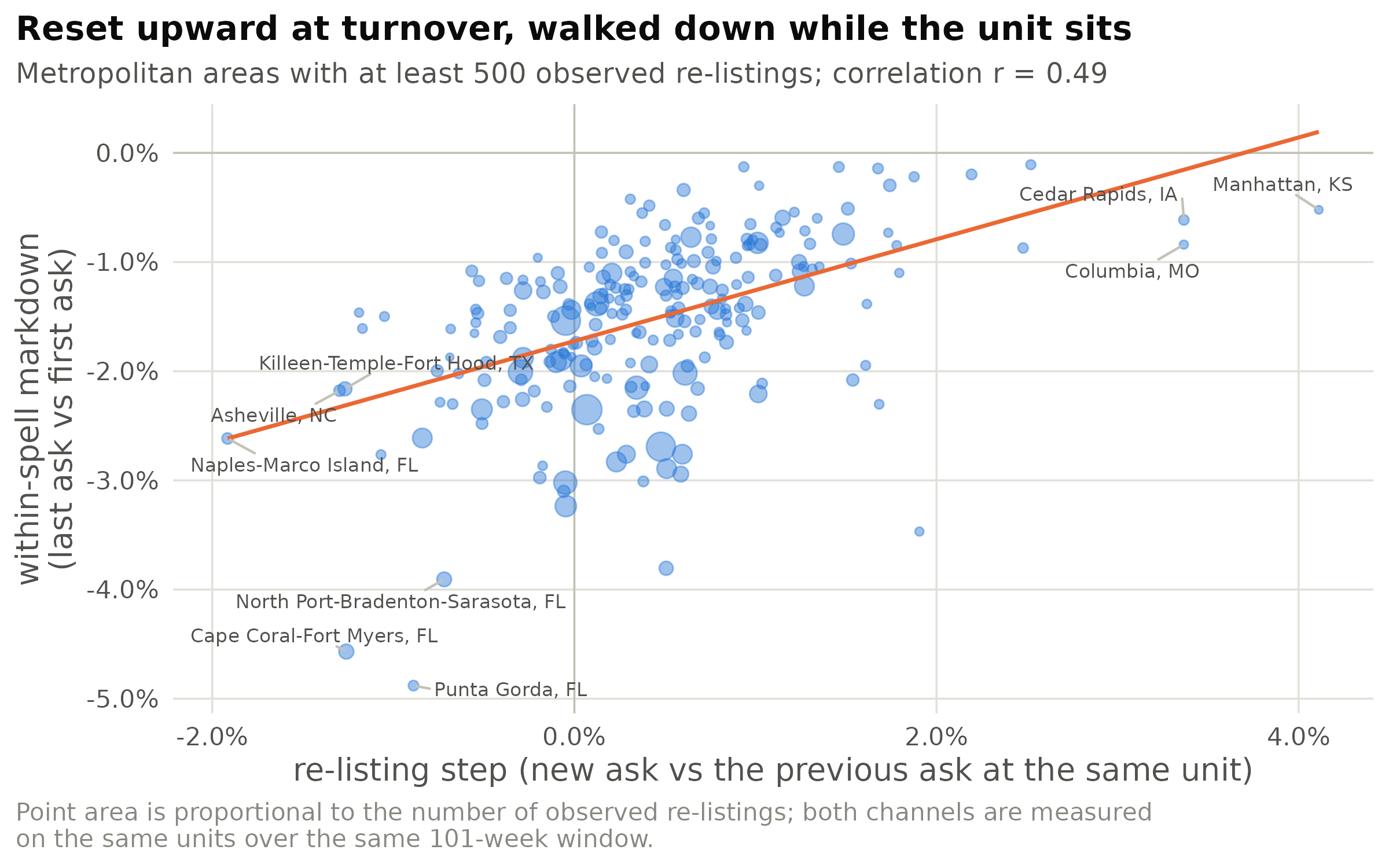
Figure 14: Each point is a metropolitan area. Landlords reset the asking price slightly upward at turnover and then give it back, several times over, while the unit sits. The two channels are positively correlated across metros, so they are not substitutes: soft markets do more of both.
The implication for index construction is real even though it did not move this level: an index built on opening asks observes only the channel that moves least when a market cools, and will therefore understate what a prospective tenant encounters. It is a reason to publish both, and not a reason to expect either to close a ten-point gap.
8. What remains: composition
Having eliminated the two explanations that could be tested inside the data, what remains is the one that cannot be: composition. The Dwellsy sample is whatever Dwellsy indexes. If the platform’s coverage tilts toward market segments, unit types, ownership structures or geographies whose rents rose more slowly than the national aggregate, then every estimator built on it inherits that tilt, which is precisely the pattern observed, with six methodologically unrelated estimators agreeing closely with one another and disagreeing with the outside world.
This is the concern Gatzlaff and Haurin (1997) formalised for repeat-sales house price indices, and their finding is directly on point: a selection-corrected index appreciated more slowly than the uncorrected one, and the difference moved with the business cycle. It is also the difference between this index and ZORI that is easiest to name. ZORI reweights its repeat-listing sample to the rental housing stock using census benchmarks for structure type, decade built and year rented (Zillow 2026); the index here applies no such correction, because the benchmark it would need does not exist for this sample.
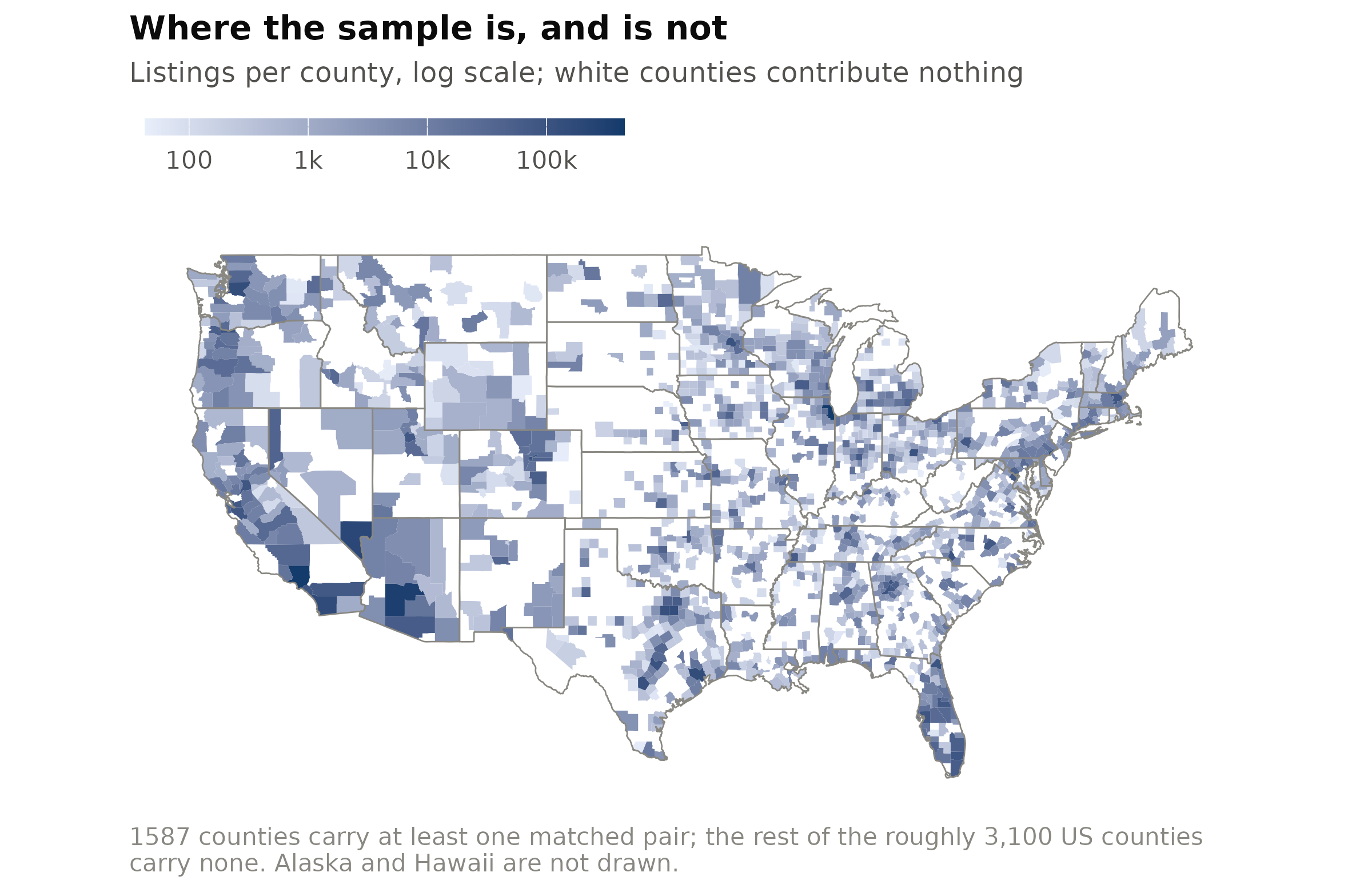
Figure 15: Listings per county on a log scale, all counties with any listing at all. The white areas are not places with no rental housing; they are places this platform does not index. Any national aggregate built from this sample weights the shaded counties and ignores the rest.
Distinguishing a tilt in this sample from the alternative (that ZORI and the CPI are themselves tilted, in the opposite direction) requires an external benchmark at the unit level, which is to say administrative or lease-level data that this project does not have. That is a limit, and it is stated as one.
9. Discussion
The index is a timing instrument, not a level instrument, and the two should be reported separately.
As a timing instrument it is validated. It recovers the turning points of the cycle, it moves a month ahead of the leading commercial asking-rent index, it moves roughly eleven months ahead of the CPI’s rent component in line with the new-tenant mechanism of Adams et al. (2024), and it orders metropolitan areas almost exactly as ZORI does. For anyone who needs to know whether the rental market has turned, several months before the official statistics say so, those are the properties that matter.
As a level instrument it is biased downward by about two percentage points a year, the bias is one-sided across all 46 metros, and (the useful part) that bias is now known not to be an artefact of the filter or of the choice of asking price.
There is a methodological lesson in the shape of the result. The dataset’s documentation identified the filter as the leading candidate for the level bias, and the identification was entirely reasonable: the mechanism is genuine, the sign is right, and the effect is estimated here at eighteen standard errors. It was simply two orders of magnitude too small. A plausible mechanism with the correct sign is not evidence of a material effect, and the distance between “this could explain it” and “this does explain it” is a dose-response curve. Truncation corrections of this kind are cheap to compute and are worth computing before a suspected bias is either corrected for or blamed.
10. Methods, data and limitations
- Estimator. Bailey-Muth-Nourse repeat-sales with Case-Shiller three-stage weighting, implemented directly on NumPy. Pair construction, the unit test and the outlier trim are identical across every band in the dose-response ladder and across every geography, so estimates differ only in the sample admitted.
- The county estimator differs from the national one. Counties use a duration-weighted mean within-unit growth rate, a period average rather than a chained index. The two are not comparable digit for digit.
- The truncation extrapolation is model-dependent. The mass outside the filter cannot be observed. A lognormal fitted to the interior gives 0.71 per cent; two alternative fitting windows give 0.92 and 0.94 per cent. Even at three times the headline estimate the correction remains under half a percentage point, so the conclusion is not sensitive to the choice, but the quantity is an extrapolation and is reported as one.
- The lead is measured in sample. Sixty-five months contain essentially one rent cycle. The eleven-month lead is consistent with an established regularity, but a claim that it will hold out of sample requires a recursive, real-time evaluation that has not been run here.
- County assignment is approximate. Counties are resolved by point-in-polygon lookup on each ZIP’s listing centroid against the same polygons the figures draw. 3.8 % of ZIPs do not resolve, mostly coastal centroids falling offshore; Alaska and Hawaii are excluded from the maps and reported in text.
- These remain asking prices. No lease, no tenant and no rent paid is observed anywhere in this data.
- Source. Dwellsy US rental listings, acquired by the University of Chicago Booth School of Business Center for Applied Artificial Intelligence. No extract of the underlying data is redistributed here; every figure reports aggregate statistics.
References
Adams, B., L. Loewenstein, H. Montag and R. Verbrugge (2024). “Disentangling Rent Index Differences: Data, Methods, and Scope.” American Economic Review: Insights 6(2): 230–245. doi:10.1257/aeri.20220685
Ambrose, B. W., N. E. Coulson and J. Yoshida (2015). “The Repeat Rent Index.” Review of Economics and Statistics 97(5): 939–950. doi:10.1162/REST_a_00500
Ambrose, B. W., N. E. Coulson and J. Yoshida (2023). “Housing Rents and Inflation Rates.” Journal of Money, Credit and Banking. doi:10.1111/jmcb.12971
Bailey, M. J., R. F. Muth and H. O. Nourse (1963). “A Regression Method for Real Estate Price Index Construction.” Journal of the American Statistical Association 58(304): 933–942. doi:10.1080/01621459.1963.10480679
Bureau of Labor Statistics (2026a). Measuring Price Change in the CPI: Rent and Rental Equivalence. bls.gov/cpi/factsheets/owners-equivalent-rent-and-rent.htm
Bureau of Labor Statistics (2026b). New Tenant Rent Index. bls.gov/pir/new-tenant-rent.htm
Center for Applied Artificial Intelligence (2026). New Datasets at Chicago Booth. University of Chicago Booth School of Business. chicagobooth.edu
Case, K. E. and R. J. Shiller (1987). “Prices of Single-Family Homes since 1970: New Indexes for Four Cities.” New England Economic Review, September/October: 45–56. NBER Working Paper 2393
Case, K. E. and R. J. Shiller (1989). “The Efficiency of the Market for Single-Family Homes.” American Economic Review 79(1): 125–137. jstor.org/stable/1804778
Cavallo, A. and R. Rigobon (2016). “The Billion Prices Project: Using Online Prices for Measurement and Research.” Journal of Economic Perspectives 30(2): 151–178. doi:10.1257/jep.30.2.151
CBRE (2025). U.S. Real Estate Market Outlook 2025: Multifamily. cbre.com
Gatzlaff, D. H. and D. R. Haurin (1997). “Sample Selection Bias and Repeat-Sales Index Estimates.” Journal of Real Estate Finance and Economics 14(1–2): 33–50. doi:10.1023/A:1007763816289
Gupta, A., V. Mittal, J. Peeters and S. Van Nieuwerburgh (2022). “Flattening the Curve: Pandemic-Induced Revaluation of Urban Real Estate.” Journal of Financial Economics 146(2): 594–636. doi:10.1016/j.jfineco.2021.10.008
Zillow Research (2026). Methodology: Zillow Observed Rent Index (ZORI). zillow.com/research