Tuning the GPU Interconnect in Multi-Node Language Model Pretraining
Contents 6 sections
Training a language model across several machines costs something that training on one machine does not. At every optimizer step, each GPU computes gradients, the corrections the model learns from, and every GPU’s copy has to be added together. On a multi-node job that sum crosses a network. This article reports what happened when I tried to make that network faster, pretraining a 2.06-billion-parameter model on two multi-node GPU clusters, each linked by a high-speed fabric, the fast network that carries traffic between nodes.
The short answer is that one change was worth a great deal, and every change after it was worth nothing, could not be measured, or crashed the job. The most useful results were therefore the negative ones. That is a common shape for infrastructure work and a rare shape for a written account of it, so the negative results are the subject here rather than an appendix.
Allocation time is billed, so every test used two nodes rather than the six the production job runs on. That sounds disqualifying, because a two-node job barely exercises the network. It is not, for a reason given in the section on scaling below, and that workaround is the most portable thing in this article.
The one change that mattered
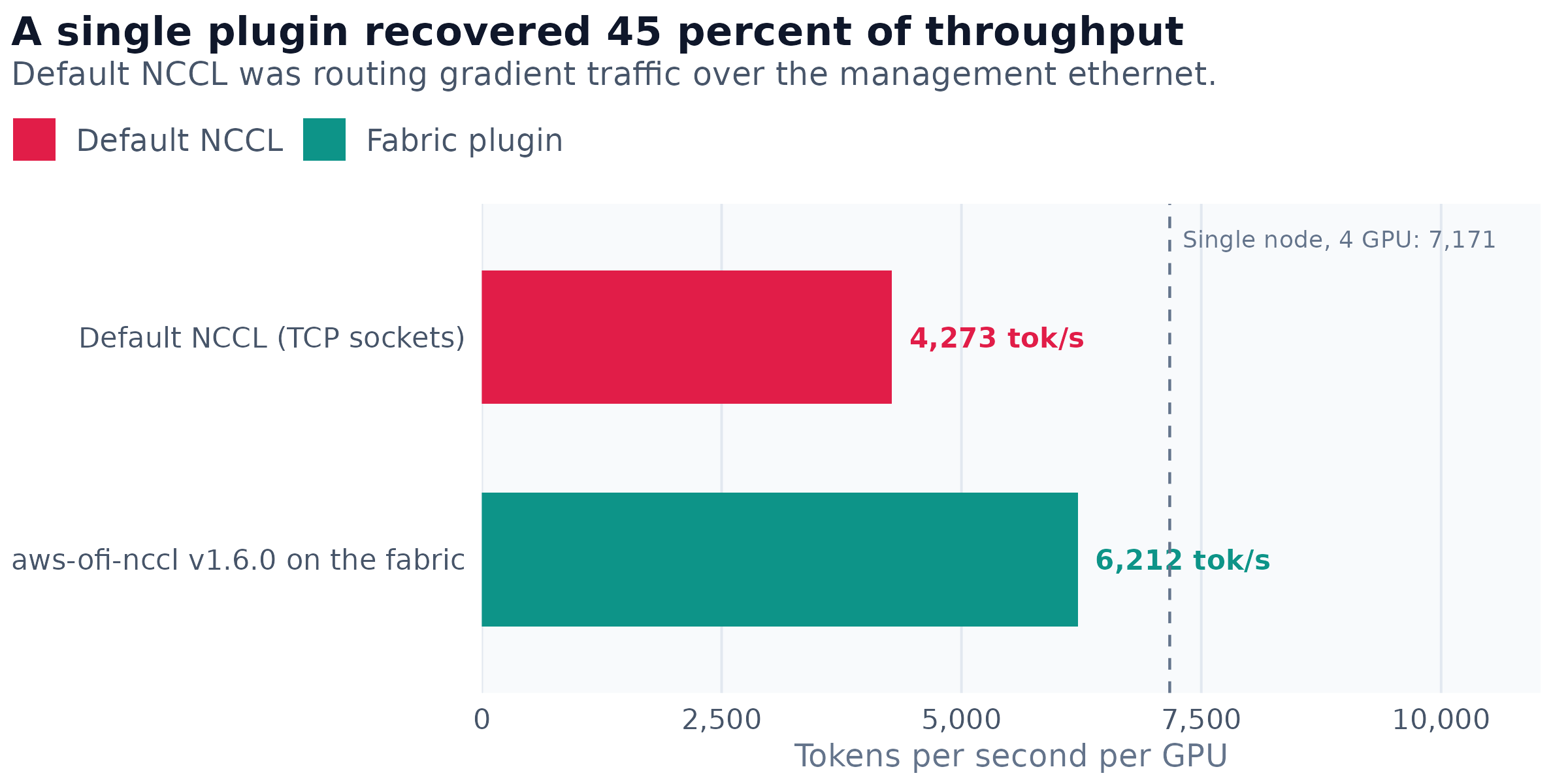
Figure 1: The single-node reference carries no cross-node traffic, so it is a ceiling rather than a controlled comparison.
NCCL, the library PyTorch uses to add gradients across GPUs, picks a network at start-up. On this cluster it picked the wrong one. With no plugin that understands the fabric, it fell back to TCP over the management ethernet, a ten-gigabit link meant for administration rather than for data. Installing aws-ofi-nccl v1.6.0 and pointing it at the fabric is the entire fix.
This is the only change from the entire exercise that reached production, and it is worth being precise: it is not a tuning result but a configuration defect. Nothing was optimized. A default was wrong, and the fix was to stop using it.
Two details cost time and are worth recording. A newer plugin, v1.9.1-aws, was worse: 1.06 GB/s on the microbenchmark against v1.6.0’s 1.92, close to the socket baseline it was supposed to replace. Newer was not better. The hypothesis that predicted it would be, that NCCL 2.27.5 advertises plugin interfaces the older build does not implement and would therefore fall back to a degraded path, was simply wrong.
Separately, requesting the Tree algorithm on its own crashes training outright, failing to find an algorithm for AllGather. A collective is one of these coordinated operations across every GPU, and the memory-saving optimizer this job uses performs collectives the microbenchmark never exercised. The production configuration names both algorithms permissively.
What the benchmark got wrong
Before touching real training I built a microbenchmark: repeatedly all-reduce a 4.1 GB buffer, the size of this model’s gradient, across eight ranks on two nodes, and time it. An all-reduce sums a value across every GPU and hands the result back to all of them; a rank is one GPU’s process. The benchmark ranked the candidate settings clearly, and it was substantially misleading about all of them.
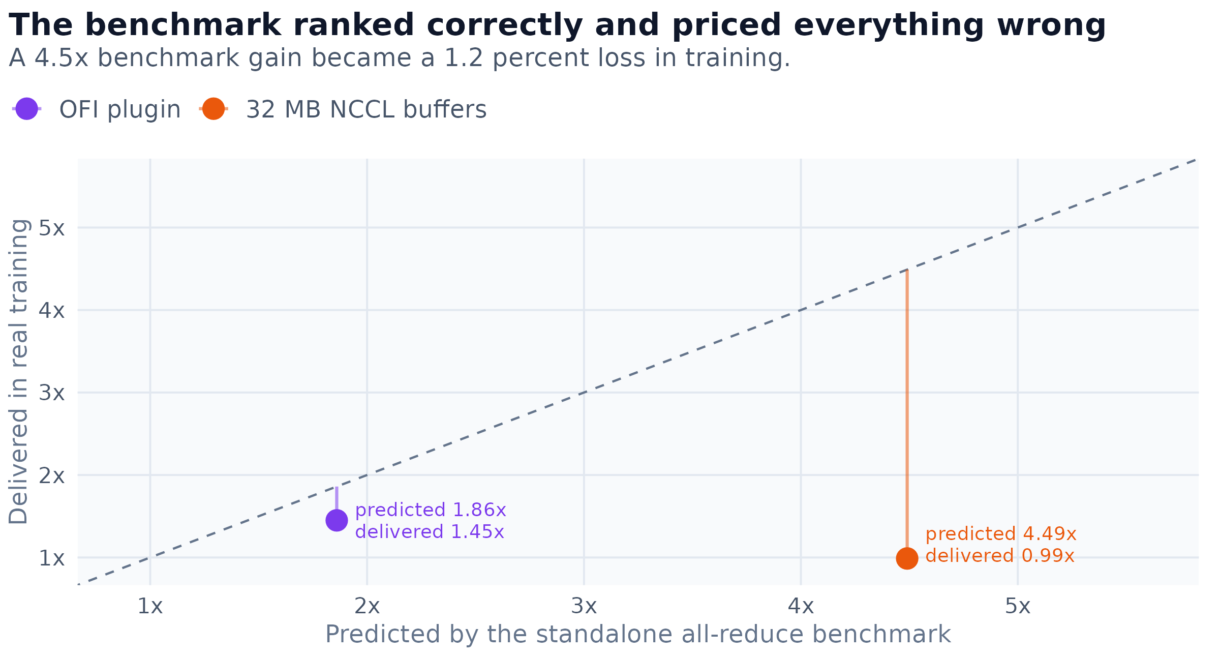
Figure 2: The dashed line is parity, where a benchmark result would transfer exactly. The Tree algorithm is absent because it crashes real training.
A standalone benchmark measures the sum in isolation, whereas in training the sum runs at the same time as the backward pass. Only the part that fails to hide behind computation shows up in the step time. The plugin’s benchmark advantage was large enough that a fraction of it still showed. Larger internal buffers made an already-hidden sum faster, which is to say they did nothing at all.
Three of the four settings the microbenchmark called wins were null or harmful in production. The lesson is not that benchmarks are useless: the ordering did survive, and ordering is what a cheap harness is for. It is that a benchmark can rank candidates but cannot price them, and the price is what decides whether to adopt.
There is a harder version of this failure, which is that for several days the benchmark had no measurement floor at all.
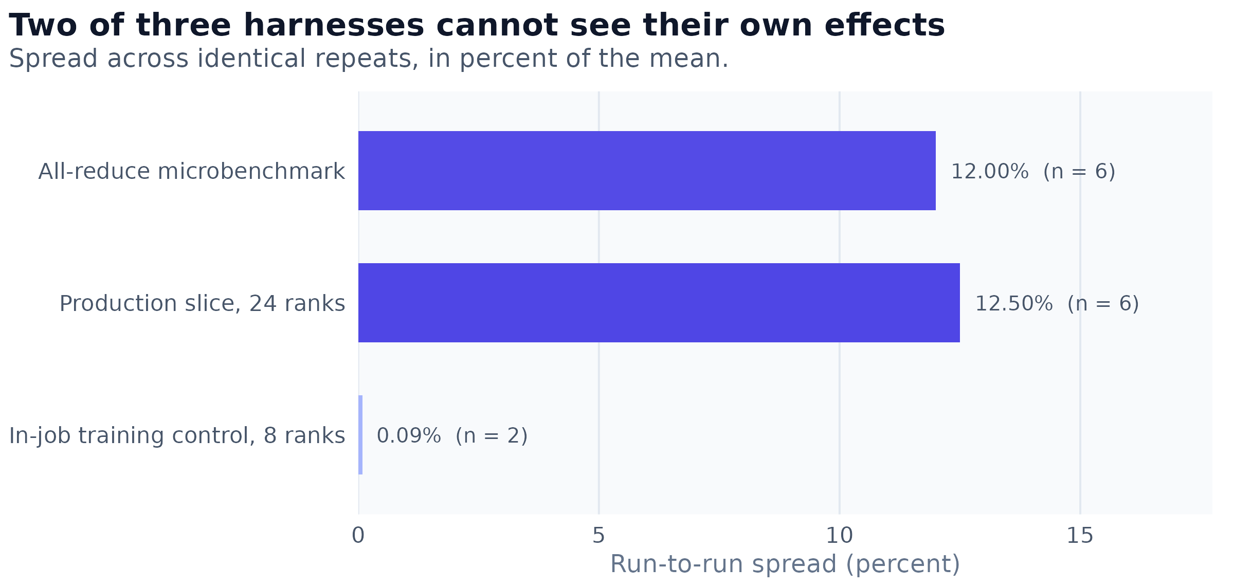
Figure 3: Any effect smaller than a harness’s own spread is unreadable by that harness.
The all-reduce benchmark’s spread across six identical runs is wider than almost every effect it was built to rank. Before that was known I had reported a 1.6 percent difference between two memory-registration settings as a ranking. It was noise. The campaign this work belongs to has an explicit rule: measure the run-to-run floor before quoting any difference. I had enforced it all week on the model experiments while exempting the benchmark, on the unexamined grounds that a benchmark is instrumentation rather than an experiment. It is an experiment.
The production slice logs have the same problem, and it is worse there, because slices are expensive and the temptation to read just one is correspondingly stronger. Two slices of the same script, at the same shape and with the same twenty-four ranks, differ by more than any effect this article reports apart from the plugin. No production claim here rests on a single slice.
The in-job control is the harness that works. Running the control arm and the treatment arm inside one allocation, each from a fresh checkpoint directory, reproduced the control almost exactly across two jobs. That precision is what makes the bfloat16 effect readable at all, and it is available only because both arms see the same node, the same filesystem contention and the same fabric neighbors.
A catalog of null results
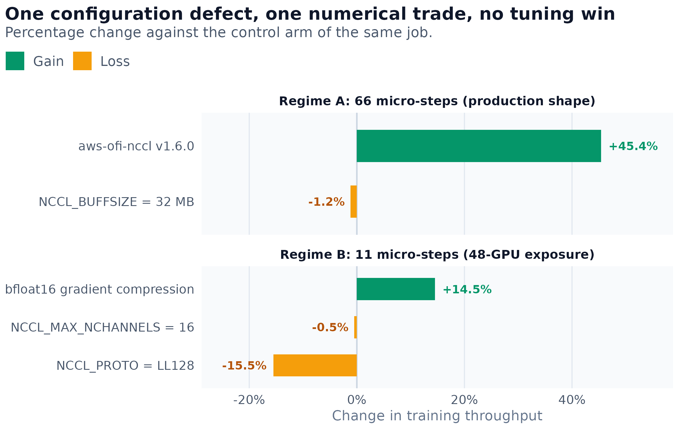
Figure 4: Each setting is measured against its own control arm in the same job. Four further settings produced no usable number and are tabulated below.
Beyond the plugin, the two settings that produced a clean number produced approximately zero.
Four settings produced no usable number at all. A gradient bucket is the chunk in which gradients are handed to the network.
| Setting | Why there is no number |
|---|---|
NCCL_ALGO = Tree alone |
Crashes: no algorithm found for AllGather |
NCCL_NET_GDR_LEVEL = PHB |
Crashes: mapping error from the fabric driver |
| DDP bucket 400 MB | Never reached steady state: memory 88.4% at step 2, 92.1% at step 3 |
| DDP bucket 100 MB | Ran, but its own control arm did not |
The 400 MB bucket is the informative failure: this job holds gradients inside the communication buckets, so a large cap demands many large contiguous regions on a card that is already nearly full. For the 100 MB bucket the only alternative to quoting no delta would be a comparison across sessions, against a slice-to-slice spread twenty-five times larger than the difference in question.
Taken singly these are unremarkable. Taken together they say something specific. At 66 micro-steps per optimizer step, the gradient sum hides so completely behind the backward pass that neither its speed, nor its algorithm, nor the number of separate transfers it is split into is observable in the step time. There is no headroom at that shape to find.
The most informative failure is the one that lost the most. LL128 is a low-latency protocol that trades bandwidth for latency, and it was the largest loss in the catalog. A configuration that gives up bandwidth to buy latency, and loses, is evidence that the regime is bandwidth-bound rather than latency-bound. That single fact retrospectively explains three earlier null results at once: bucket size did nothing because transfer launch latency was never the constraint, and the Tree algorithm’s fewer network hops bought nothing for the same reason. A negative result used as an instrument is worth more than the positive result it was hunting.
One qualification keeps that from being tidy. If the link were simply starved of bandwidth, raising the number of parallel communication channels should have helped, and it did not. The defensible statement is that the regime is bandwidth-bound at the level of the payload rather than starved of channels.
How much of a step is communication
Every estimate in this campaign of the fraction of step time spent communicating had been an inference. One measurement finally produced a number, from the only intervention that reduced how much data was sent rather than how fast it was sent.
Summing gradients in bfloat16, a 16-bit number format, rather than in 32-bit single precision halves the bytes on the wire. It returned 14.5 percent, not 100 percent. Solving for the communication fraction gives approximately 25 percent of step time in the exposed regime, of which halving the payload recovered half. The arithmetic is elementary; the point is that it is arithmetic on a measurement rather than on an assumption.
This result is not adoptable on throughput evidence alone, which is why it is reported separately from the others. Every other setting in this article is quality-neutral by construction: changing which network carries a sum, or how it is chunked, cannot change the sum. Compressing gradients before summing them changes the arithmetic the model trains on. The comparison that would settle it is a matched pair of runs differing only in this setting, read on training loss rather than on throughput.
That comparison has not produced a valid result. Its first attempt was void, for a reason worth recording because it will recur in anyone’s short probe derived from a long training script. It inherited --warmup_steps 8000 from the production command. Within the roughly twenty-five steps a short wall-clock limit allows, the learning rate therefore never exceeded about 1.9e-6, the weights had barely left their initialization, and both arms reported a loss identical to four decimal places. Two nearly untrained models cannot diverge numerically, whatever precision sums their gradients. Any probe derived from a production configuration must override the production warmup schedule, or it measures initialization.
What does not scale
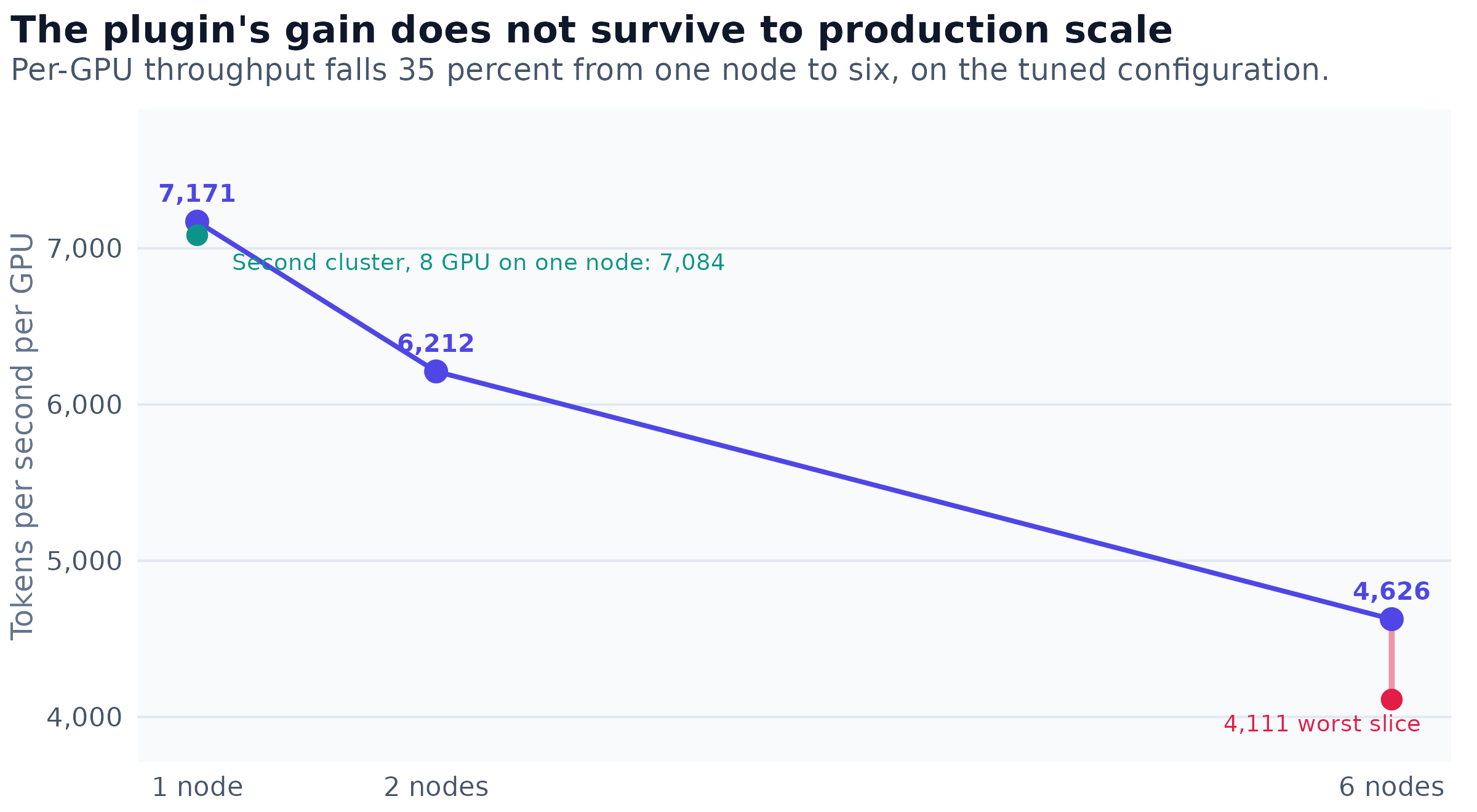
Figure 5: The six-node point shows the best and the worst of six slices at one fixed configuration.
The per-GPU cost of spanning nodes grows from roughly 13 percent at two nodes to roughly 35 percent at six. Two-node results can therefore rank candidate settings but cannot size the win, so every number in the sections above should be read as a ranking.
The obvious alternative explanation can be ruled out. The two clusters are within about a percent of each other on a single node, they use the same generation of accelerator, and neither configuration crosses a node. Per-GPU compute is effectively identical on the two machines, so the decline across the series is communication and not hardware.
One correction belongs here rather than in a footnote, because I quoted the affected number repeatedly before checking it. The two-node figure of roughly 13 percent is confounded. The single-node reference runs 132 micro-steps per optimizer step and the two-node measurement runs 66, because the same global batch is divided among twice as many devices. Halving the micro-step count halves the window available to hide the sum, which is a throughput cost with no network involvement whatsoever. I attributed the entire gap to crossing nodes. The control that separates the two effects needs a single node, so that it contains no cross-node traffic at all, and must vary only the micro-step count by shrinking the global batch. It has not been run.
That same relationship is why two-node testing was viable. The number of micro-steps is the global batch divided by the number of devices, and both terms are chosen by the experimenter rather than imposed by the hardware. Shrinking the batch on two nodes reproduces the micro-step count, and therefore the collective exposure, of a job six times the size. Regime B in the catalog above is exactly that: an eight-GPU job configured to expose its communication the way a forty-eight-GPU job would. Buying twelve nodes to discover that a setting is null is avoidable.
What remains open, and what to take away
Three questions are unresolved. The single-node micro-step control has not been run, so the split between crossing nodes and dividing the batch remains unmeasured. The quality of bfloat16 gradient compression, the only remaining lever with a measured gain, is unvalidated. And the exposed cost at production scale has not been broken down: the candidates that no transport setting would touch include reading training data from a shared filesystem, checkpoint writes, and slow individual ranks holding up each collective.
The transferable conclusions are narrower than the effort behind them, which is the usual result and worth stating plainly.
Check that the library chose the right network before tuning anything about how it uses that network. The one large win here was a wrong default rather than a badly chosen parameter, and it was invisible in every metric except aggregate throughput.
Measure the reproducibility of a harness before quoting a difference it reports. Two of the three harnesses used here have a spread wider than most of the effects they were asked to resolve, and both were used in that state before anyone checked.
Prefer a control in the same job to a remembered number from a previous one. The two extremes of Figure 3 are the same measurement of the same configuration, differing only in whether the comparison shared an allocation.
Reproduce the regime rather than the scale. A collective that hides completely behind computation can be neither optimized nor measured; one deliberately exposed can be both, and exposing it is a matter of arithmetic on the batch shape rather than of buying nodes.
Finally, these results describe one fabric, one model size and one framework. The plugin defect is likely to generalize wherever a specialized interconnect meets a library that does not recognize it. The catalog of nulls almost certainly does not: a job with fewer accumulation steps, a larger model, or a slower network would expose its communication differently, and the settings that were unreadable here would become readable there. The method is the portable part.