Evaluating AI Agents When Every Run Differs: Repeated Trials, Paired Comparisons and Graders
Contents 10 sections
- Why agents are harder to evaluate than models
- One run is one draw
- Compare two agents on the same tasks
- Several runs per task, step by step
- How many tasks, and how many runs
- Graders: how a run gets its score
- Where the test cases come from
- When offline and online disagree
- Catching regressions before release
- Conclusion
An agent that completes a task today may fail the same task tomorrow, so a single run of an evaluation is one draw from a distribution rather than a measurement of the agent. Comparing two versions of an agent therefore needs the tools of an experiment: repeated trials, comparisons made on the same tasks, an interval around every difference, and graders whose own errors are known. This article sets out each of them, using a simulated pair of agents whose true difference is known in advance, so that it is possible to see when an evaluation finds the truth and when it does not.
Why agents are harder to evaluate than models
A classifier gives the same answer to the same input every time, so it can be scored once. An agent does not, for three reasons. The model samples each token with some randomness, so its plan, its tool calls and its final answer can change from one run to the next; even a temperature of zero does not make a hosted model repeatable, for reasons set out in an earlier article on this site. The tools and environments change: a web page is updated, an API times out, a file system is in a different state, and the agent reacts to what it finds. And many tasks have several right answers, so checking for one exact output fails correct runs that took another route.
An agent’s result on a task is therefore not a fact about the agent. It is one draw from everything the agent might have done.
One run is one draw
Suppose an agent succeeds on a particular task with probability p on each try. Three measures describe it, and they answer different questions. pass@1 is p itself: how often a single try succeeds. pass@k is 1 − (1 − p)k: how often at least one of k tries succeeds, the right measure when a person or a test can pick out the one good attempt, as when several candidate patches are generated and the one whose tests pass is kept. pass^k is pk: how often all k tries succeed, the right measure when a user depends on the agent working every time, as with a support agent that issues refunds.
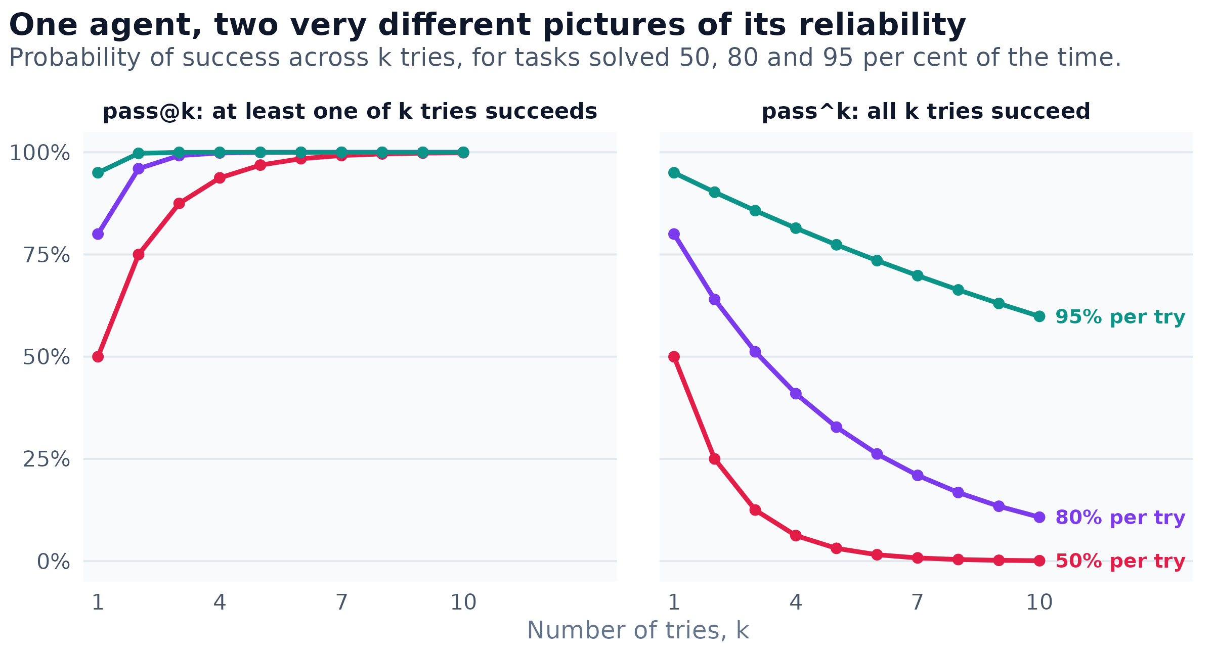
Figure 1: Exact values for a single task with a fixed success rate per try.
pass@k flatters and pass^k is honest about reliability. The pass^k measure was introduced by τ-bench, a benchmark in which an agent serves a simulated customer under a company’s written policy and is graded on the state of the database when the conversation ends. Its published leaderboard shows the measure at work on real agents.
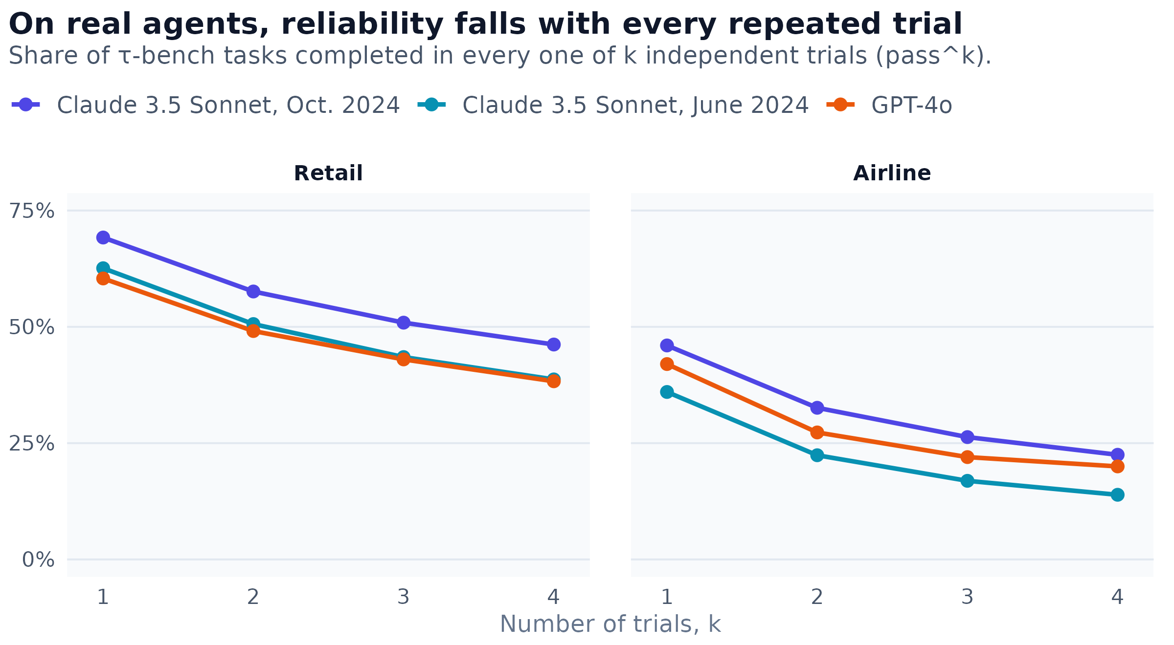
Figure 2: From the τ-bench leaderboard, tool-calling agents. Retail and airline are the benchmark’s two domains of customer-service tasks.
The best of these agents completes fewer than half of the retail tasks in all four of four tries. The curves also fall more slowly than pk would predict from their first points, because tasks differ: some are solved every time and some never, and those tasks do not decay. That spread of difficulty matters for everything that follows, so the simulated agents in this article are built to share it. Each simulated task has its own success rate, and the spread of those rates is fitted so that the population reproduces GPT-4o’s retail scores above (the fit is within 0.3 points at every k). The second agent, B, is better than the first, A, by exactly 6 points on average, by an amount that varies from task to task.
Compare two agents on the same tasks
The most useful single habit is to run both agents on the same tasks and compare them task by task, which is called a paired comparison. Tasks differ in difficulty far more than two versions of an agent differ from each other. If A and B ran on different tasks, B could look better merely by drawing easier ones; pairing removes that, because every task is compared with itself.
With one run of each agent per task, the comparison reduces to a table of four cells. Suppose, for illustration, that A passes 30 of 50 tasks and B passes 34:
| B passed | B failed | |
|---|---|---|
| A passed | 28 | 2 |
| A failed | 6 | 14 |
On 42 tasks the two agents agree, and those tasks say nothing about which is better. All the evidence lies in the 8 tasks where they disagree, of which B won 6 and A won 2. McNemar’s test asks how surprising such a split would be if the agents were equally good, and the answer is not very: a split at least as uneven as 6 to 2 arises by chance 29% of the time. An eight-point gap in the headline rates is not yet evidence.
The difference pairing makes is easiest to see in simulation. The next figure repeats the same evaluation of the simulated agents ten thousand times, once with both agents on the same 50 tasks and once with each agent on its own 50.
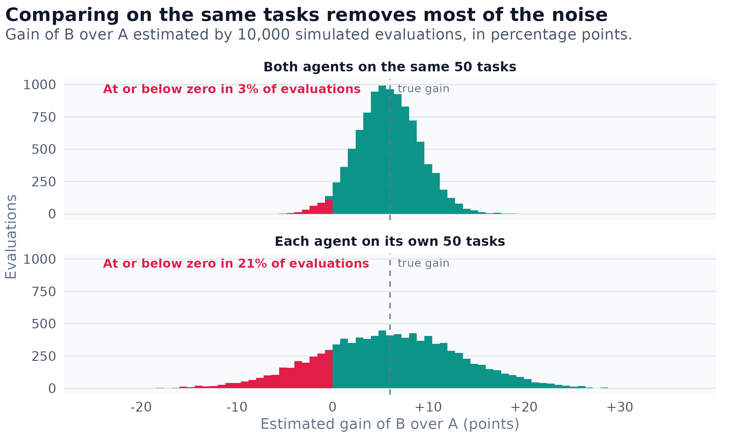
Figure 3: Simulation. Each evaluation runs each agent 5 times on each of 50 tasks drawn from the population described above; 10,000 evaluations per design.
The two designs cost exactly the same, five runs of each agent on 50 tasks, and the unpaired one points the wrong way about seven times as often. Nothing about the agents changed: only whether their tasks were shared.
Several runs per task, step by step
With several runs per task, a task no longer simply passes or fails. Each agent has a success rate on it, such as three passes in five, and the analysis works on those rates. The procedure below follows the recommendations of Miller’s statistical guide to evaluations: infer from the task-level paired differences, and plan the size of the evaluation in advance.
- One row per task. Record how many runs each agent passed and the difference between their rates. The task is the unit, not the run: the five runs of one task share its difficulty, so they are five looks at one thing rather than five independent pieces of evidence. Treating 250 runs as 250 tasks makes the result look far more certain than it is.
- The effect size. Average the per-task differences over every task, ties included. Dropping the tied tasks would inflate the gain, since on those tasks B is no better.
- A confidence interval by bootstrap. Draw 50 tasks at random from the 50, with replacement, each bringing its whole row so that the pairing is kept; average the differences; repeat 10,000 times; and keep the middle 95 per cent of the averages.
- A second opinion from the signed-rank test. The Wilcoxon signed-rank test ranks the non-zero differences by size and asks whether B’s wins outrank A’s. It makes no assumption that the differences follow a bell curve, which they rarely do: here they come in steps of 20 points, and many tasks sit at zero.
- The tasks B lost. The average hides losses. A version that newly breaks an important task is not better, however the average moved, so the worst tasks deserve to be read run by run.
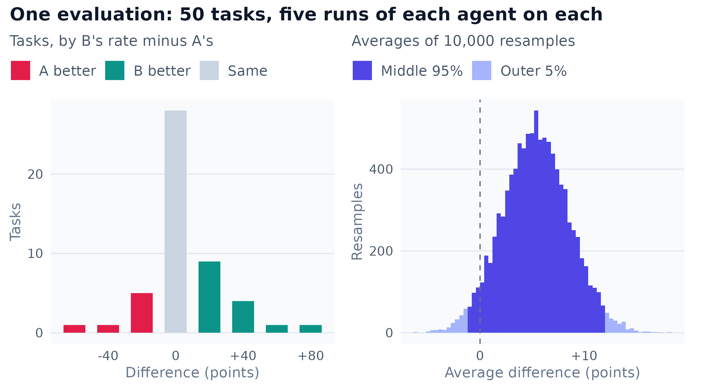
Figure 4: Simulation: the first evaluation of the agents described above, with the seed fixed before it was run. The interval is the middle 95 per cent of 10,000 bootstrap averages.
Written up, this evaluation reads:
B scored 5.6 points higher than A (95% interval −0.8 to 12.0 points; signed-rank p = 0.09), over 50 tasks run 5 times by each agent. B did better on 15 tasks, worse on 7 and the same on 28; its worst loss was 60 points.
That sentence carries the size of the difference, how far it can be trusted, how much evidence it rests on and where it went wrong, which “B won 15 tasks to 7” does not. And its honest conclusion is that the evaluation has not settled the question. The interval reaches below zero and the test does not reach significance, so the data allow anything from a small loss to a clear gain. That is “not known yet”, which is different from “no difference”, and in this case it is wrong to read it as either: the simulation was built with a true gain of 6 points, and this evaluation was simply too small to establish it.
Repeated runs also yield pass^k directly. With five runs per task, pass^5 is the share of tasks on which all five runs passed: 28% for A and 32% for B here, with a 95 per cent interval on the gap from −4.0 to 12.0 points. Scoring each task as all or nothing discards information, so a claim about reliability needs more tasks than a claim about average success. For smaller k the same counts serve: a task passed in 4 of its 5 runs contributes 4 in 10 to pass^3, because 4 of the 10 ways of choosing three of its runs choose only passes, the reliability counterpart of the unbiased pass@k estimator used for code models.
How many tasks, and how many runs
Two kinds of noise blur an average: tasks differ from one another, and every run has its own luck. A new task averages out both, while an extra run averages out only the second. The next figure asks how often evaluations of different shapes detect the simulated agents’ true gain, holding fixed the total number of runs each agent receives.
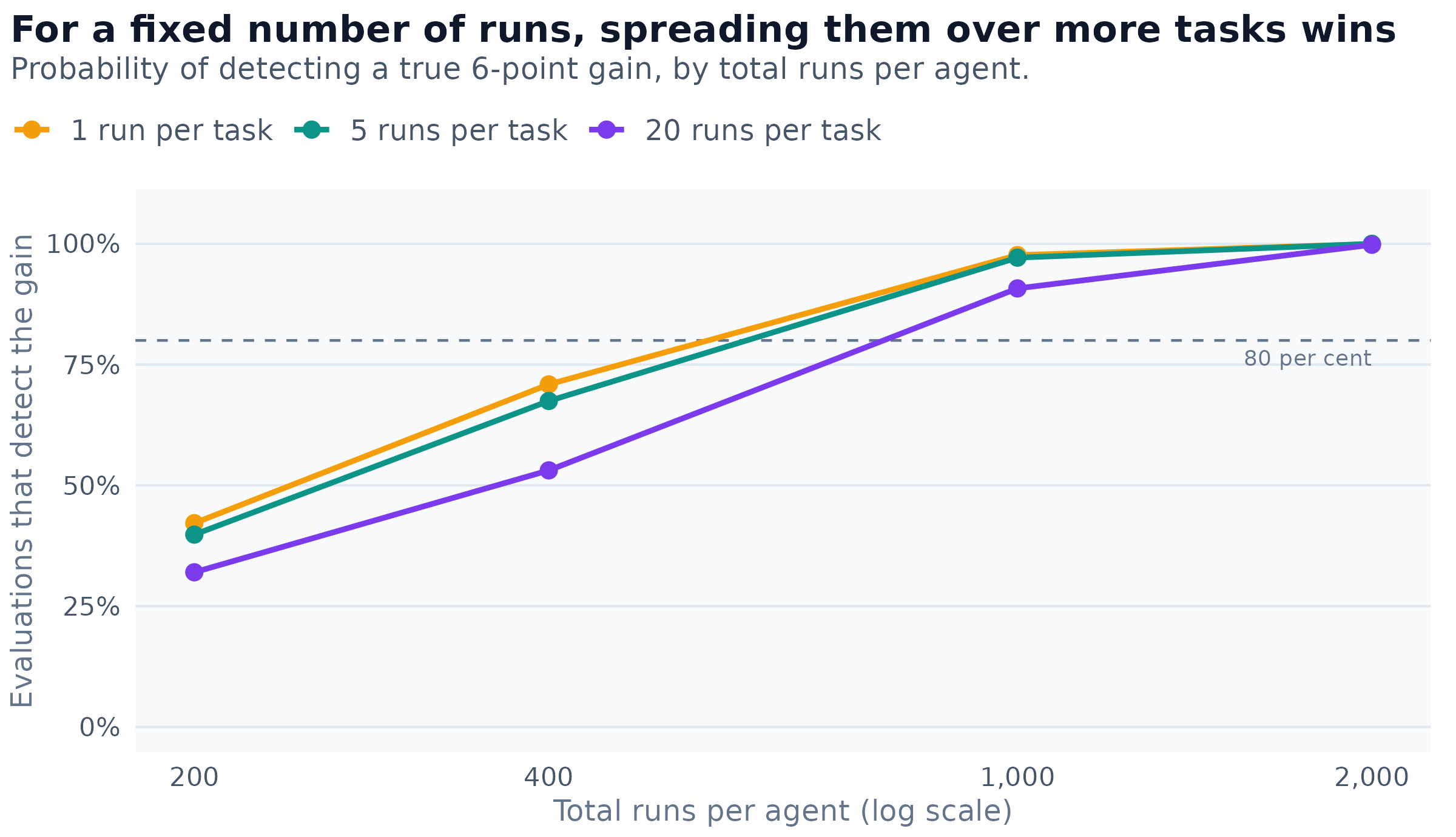
Figure 5: Simulation: 3,000 evaluations per point, each detecting the gain when its 95 per cent interval (the mean difference plus or minus 1.96 standard errors) lies above zero. At 1,000 runs, for example, the three designs use 1,000, 200 and 50 tasks.
The evaluation in the previous section, 50 tasks with five runs each, would sit on the five-run line between its first two points. The same simulation puts its chance of detecting the true gain at 47%, so its inconclusive result was unremarkable rather than unlucky. For a given budget of runs, more tasks is the better use of it, even at a single run each. Several runs per task remain worth having for what they add beyond the average, a measure of each task’s reliability (pass^k) and a view of which tasks are erratic, and when the task set is fixed, as it usually is because good tasks with a reliable checker are expensive to build, extra runs are the remaining way to sharpen the result. Either way, both numbers should be fixed before the evaluation starts. Adding tasks until the interval clears zero and then stopping turns luck into a result.
Graders: how a run gets its score
Every evaluation needs a way to decide whether a run succeeded, and there are three kinds of grader. The best evaluations use the cheapest one that is reliable for each task.
| Grader | Suited to | Characteristic failure |
|---|---|---|
| A deterministic check: tests pass, a record has the right value | anything with a checkable end state | a weak check passes a wrong answer, such as a test suite that never exercises the bug |
| A person with a rubric | subjective quality, safety review, building a reference set | slow and costly, and people disagree with one another |
| A language model as judge | open-ended answers at scale | biases of its own, described below |
Wherever possible, grade the end state rather than the path. A long task can be solved in many ways, so check what the agent achieved (the ticket is closed, the booking exists exactly once, the report cites real sources) and check the path only for rules that must never be broken, such as calling a forbidden tool. τ-bench grades this way, comparing the database at the end of each conversation with the state the task should have produced. Tools with side effects need the same care: anything that sends, pays or deletes is mocked or sandboxed during evaluation, and a long task’s environment is restored from a snapshot so that every run and every agent starts from the same state.
A model used as a judge is convenient and measurably biased. Zheng and colleagues found that strong judges agree with human preferences about as often as people agree with each other, above 80 per cent, and also that every judge they tested favoured an answer partly because of where it appeared.
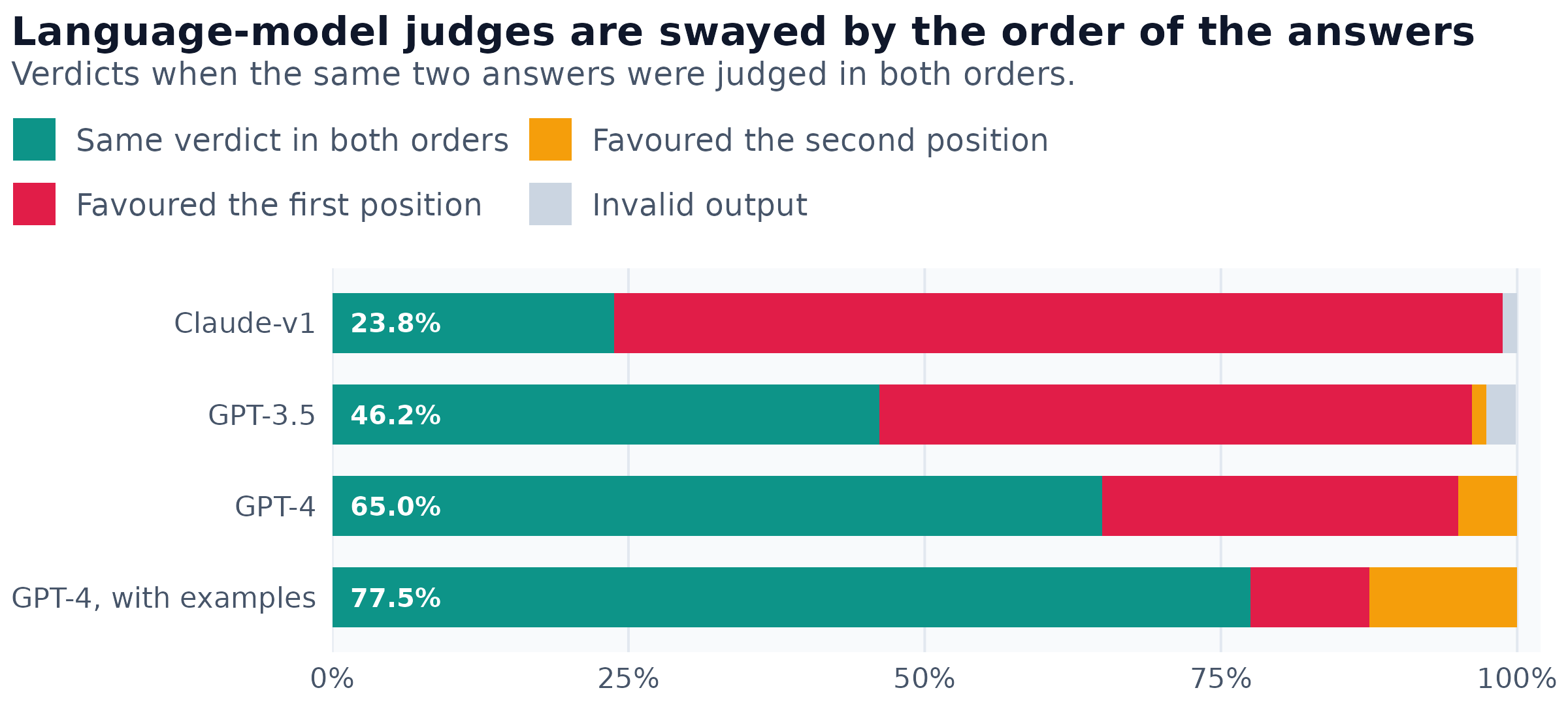
Figure 6: From Zheng et al. (version 4), Table 2 and the few-shot table in its appendix. Each judge compared the same pairs of answers twice, with their order swapped.
Position is one of several biases, and each has a counter. A judge that favours a position is asked twice, with the order swapped, as in the figure. A judge that favours longer, more polished or more confident answers is given a rubric that scores specific facts. A judge that favours its own model family, a bias Panickssery and colleagues traced to models recognizing their own writing, is replaced by a judge from another family, with the authorship hidden. Above all, a judge is validated before it is trusted: people label a few hundred outputs, the judge grades the same ones, and their agreement is measured separately for each agent being compared. A judge that agrees with people more often on one agent’s answers than another’s is tilting the comparison.
Even an unbiased grader with ordinary error distorts a comparison in a predictable way. If it passes a successful run with probability s and wrongly passes a failed one with probability f, every measured difference between two agents is the true difference multiplied by s − f. A grader that catches 95 per cent of successes and passes 10 per cent of failures shrinks every gap by 15 per cent, which makes real improvements harder to detect; and a grader whose errors differ between the two agents can manufacture a gap where none exists.
Where the test cases come from
Without production traffic, an evaluation starts small and hard: a few dozen cases written from the specification with an expert, favouring the tricky ones, and every failure met while trying the agent by hand. Cases can be generated by a model, but each needs checking by hand, because a generated case with a wrong expected answer grades the agent against a mistake. Reading failed runs and sorting them into kinds of failure should come before deciding what to count; a metric chosen before anyone has seen the failures often measures the wrong thing. A held-out set that is never used while tuning prompts keeps the suite honest, because a suite tuned against stops predicting performance on new cases.
Public benchmarks add the risk of contamination: a benchmark that leaked into a model’s training data measures memory rather than skill. When Zhang and colleagues wrote a fresh set of grade-school arithmetic problems matched in style and difficulty to the widely used GSM8k, the accuracy of some model families fell by up to 8 per cent on the new problems. Rewriting test items with the same meaning in new words, or writing new ones after a model’s training cutoff, is the corresponding check for any suite.
When offline and online disagree
An offline evaluation is a test suite. Online evaluation is what users experience: tasks completed, escalations, retries, corrections, abandoned sessions. When the suite says a new version is better and users say it is worse, the users should be believed first and the suite treated as the suspect. The usual causes are four. The test set no longer resembles real use, which a comparison of the real mix of requests with the suite’s will show. The judge is being gamed, because the new version has learned what the judge rewards (length, tone, confidence), which fresh human labels will reveal. One segment of users got worse while the average rose, which only a breakdown by segment exposes. Or something other than quality changed, such as slower answers, more clarifying questions or higher cost, which latency and turn counts beside the quality metric will show.
Catching regressions before release
Every prompt change and every model swap produces a new agent. A release gate turns “is it at least as good?” from an impression into a check that can fail:
- a fixed suite, paired: the new version against the old on the same tasks, several runs each, with an interval on the difference;
- recent real traces: a fresh sample of real requests, replayed or mocked, so the suite does not go stale;
- guardrail metrics: safety violations, cost per task and latency, which must not get worse even when quality rises, the point Kapoor and colleagues make about benchmarks that report accuracy alone;
- the worst task as well as the average: a version that is better on average but newly fails an important task is not better;
- a way back: the old version can be restored quickly if online metrics fall.
Conclusion
An agent’s score on an evaluation is a sample, and the methods that make samples informative are old and well tested: repeat the trials, compare on the same units, report an interval, and decide the size of the experiment before running it. The simulation in this article had the advantage of knowing the truth, and it shows how easily an honest evaluation of a realistic size can fail to see a real 6-point improvement, and how often a careless one points the wrong way. The interval, with the number of tasks and runs beside it, is the result worth reporting; a win count or a single headline rate is not.