Argonne 3.5-base: Retraining an Unchanged Architecture With a Revised Recipe

What was changed, and what was not

The architecture is unchanged: 24 layers, hidden size 3,072, 12 query and 4 key-value attention heads, a SwiGLU feed-forward network, RMSNorm with query/key, value and sandwich normalizations, a logit softcap, rotary position embeddings, and tied input/output embeddings — 2,882,162,688 parameters, described in the earlier article. What changed is everything around it.

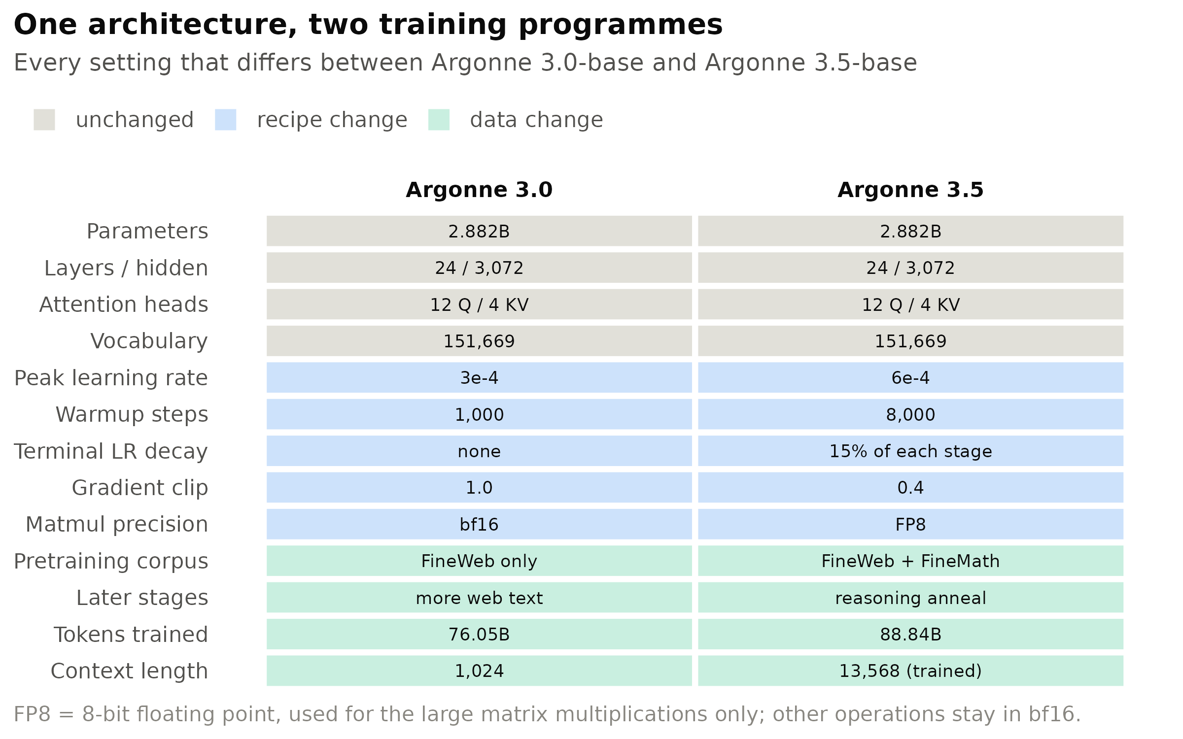
Figure 1: Grey cells are identical between the two versions; coloured cells changed. The architecture rows are unchanged by design, so the two models differ only in how and on what they were trained.

The recipe rows are the subject of the next section, and the data rows of the one after it.

The decay phase that was missing

The most consequential change is also the least conspicuous, and it began as a defect rather than an idea.

Argonne 3.0 used a warmup–stable–decay learning-rate schedule. The learning rate governs how large a correction the model makes at each of its hundreds of thousands of update steps; the standard practice is to raise it quickly, hold it at a plateau for the bulk of training, and then anneal it toward zero at the end, so that the final weights settle rather than continue to jump around. The decay phase is where a large part of the quality gain lives.

Argonne 3.0 never performed it. Its launcher passed a decay length of zero, and the scheduler interpreted zero as “return a constant” — so the plateau ran to the last step of the run and the model was exported at full learning rate. The setting intended to soften the ending silently removed it.

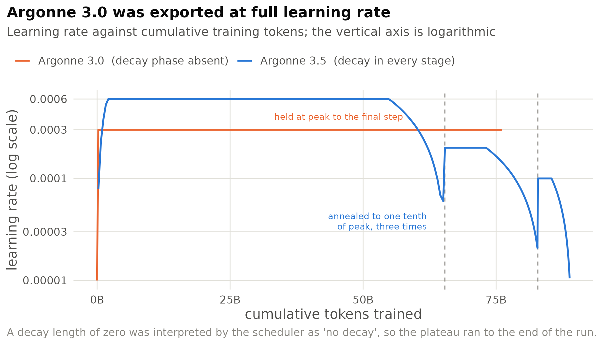
Figure 2: Argonne 3.0’s schedule is reconstructed from its launcher flags and the scheduler source; Argonne 3.5’s is read from its own training logs. Vertical dashed lines mark 3.5’s stage boundaries.

The correction is worth its own measurement, because it was made mid-flight: Argonne 3.5’s first stage did decay, its second stage inherited the same zero and did not, and it was corrected while that stage was running. Held-out cross-entropy was measured on eight subject-matter categories before and after the first stage’s decay phase: every one improved by 0.12 to 0.34 nats, including categories the stage never trained on, and that decay phase alone out-earned the entire 175,000-step plateau preceding it. That is the size of the effect Argonne 3.0 forfeited.

The second stage made the case concrete in the other direction. Measured mid-stage, while still at constant learning rate, it was improving on every one of its target subjects and simultaneously losing general knowledge: held-out cross-entropy on general educational text rose by 0.25 nats, far enough that Argonne 3.0-base was briefly the better model on it, despite that text making up 9% of the mixture — the other 91% simply swamped the replay. Restoring the decay reversed it, and by the first post-decay checkpoint all eight categories were ahead of Argonne 3.0-base again.

Two further observations belong with this. During a constant-rate plateau the weights are demonstrably not settling: five checkpoints taken 1,200 steps apart swing 0.62 nats on the same held-out text, simply tracking whatever the most recent batches contained. And the identical defect later appeared in a successor project, because the fix had been applied in one working copy of the launcher and not the other — a reminder that a repository with two checkouts has two configurations.

The three remaining recipe changes are smaller and were carried over from a proxy-scale search conducted before the run: the peak learning rate was doubled to 6e-4, the warmup lengthened eightfold to match it, and the gradient clip tightened from 1.0 to 0.4. The last is what makes the first safe — a tighter clip curbs the larger updates a higher learning rate produces — and none of the three is a change in what the model is, only in how hard it is pushed.

Numeracy designed in, rather than repaired afterwards

Argonne 3.0-base was trained on FineWeb, a filtered snapshot of the open web. It emerged fluent and broadly knowledgeable and unable to compute 8 + 3. The reasoning work that followed spent months repairing this: a corrective training stage on mathematical text, then a linear average of two checkpoints to reconcile the mathematics it gained against the general knowledge it lost.

Argonne 3.5 mixed mathematics into pretraining from the first step instead — FineMath at 15% of the corpus, FineWeb at 85% — and then followed it with two further stages on progressively more specialised data.

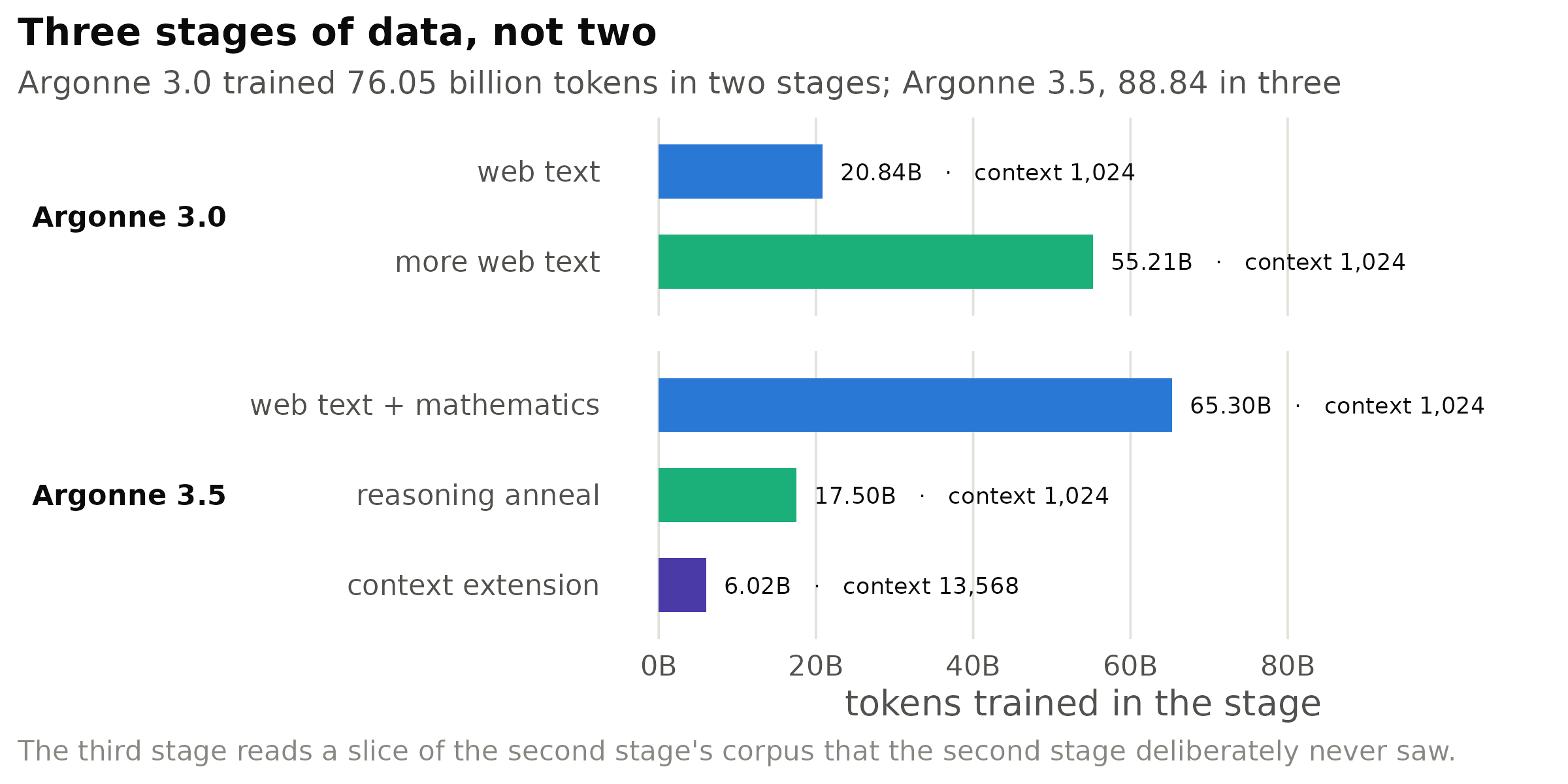
Figure 3: Bar length is tokens trained in that stage; the label gives the token count and the context length at which the stage ran. Argonne 3.5 trained on 17% more text, in three stages rather than two.

The second stage, an anneal, trains on a mixture of code, mathematics, reasoning traces and tool-use transcripts, with a smaller replay tier of general educational text to guard against forgetting. The third stage takes a deliberately disjoint quarter of that same corpus — reserved before the second stage began, so no reasoning token is trained on twice — and reads it at a context of 13,568 tokens instead of 1,024.

A cheap probe tracked whether the mathematics was arriving: 20 arithmetic and word-problem questions and 15 general-knowledge questions, graded by exact match, run on intermediate checkpoints for about ten GPU-minutes each. Its purpose was a go/no-go decision — whether the base was worth the expense of a reasoning recipe — not a capability measurement.

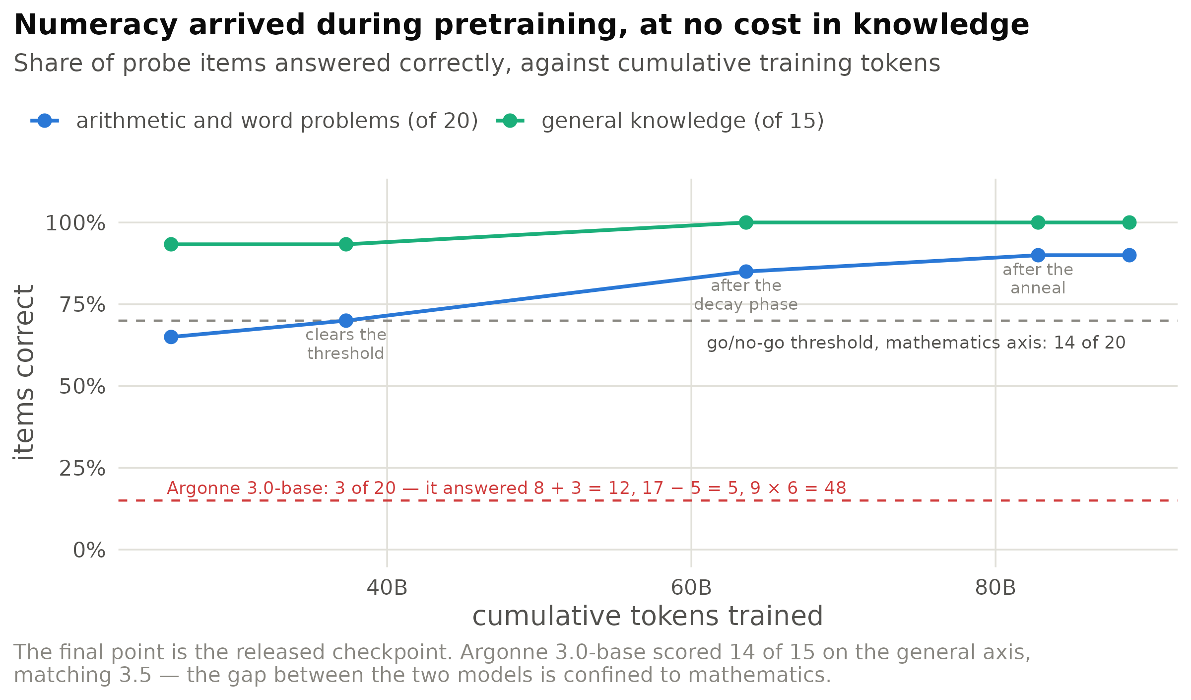
Figure 4: A 35-item probe, greedy decoding, run on live checkpoints. The probe has a measured noise floor of about two items and saturates, so it certifies readiness rather than measuring capability.

A controlled comparison isolates the cause. The same probe, the same grader, the same architecture and tokenizer were applied to a freshly downloaded Argonne 3.0-base: 3 of 20 on mathematics, 14 of 15 on general knowledge. At the point Argonne 3.5 crossed the threshold it had seen roughly 5.8 billion interleaved FineMath tokens, and that interleaving was the only substantive difference between the two corpora. The remaining misses are also different in kind: Argonne 3.0-base failed single-digit arithmetic, while Argonne 3.5’s failures are multi-step and formulaic — solving for a variable, a rectangle’s perimeter, a factorial.

Two honest limits. The probe is small, curated and saturating, and a separate few-shot evaluation on standard benchmarks read close to chance on this checkpoint, so it should not be read as a claim of broad capability. And no standard held-out benchmark suite has yet been run on the released base.

The training record

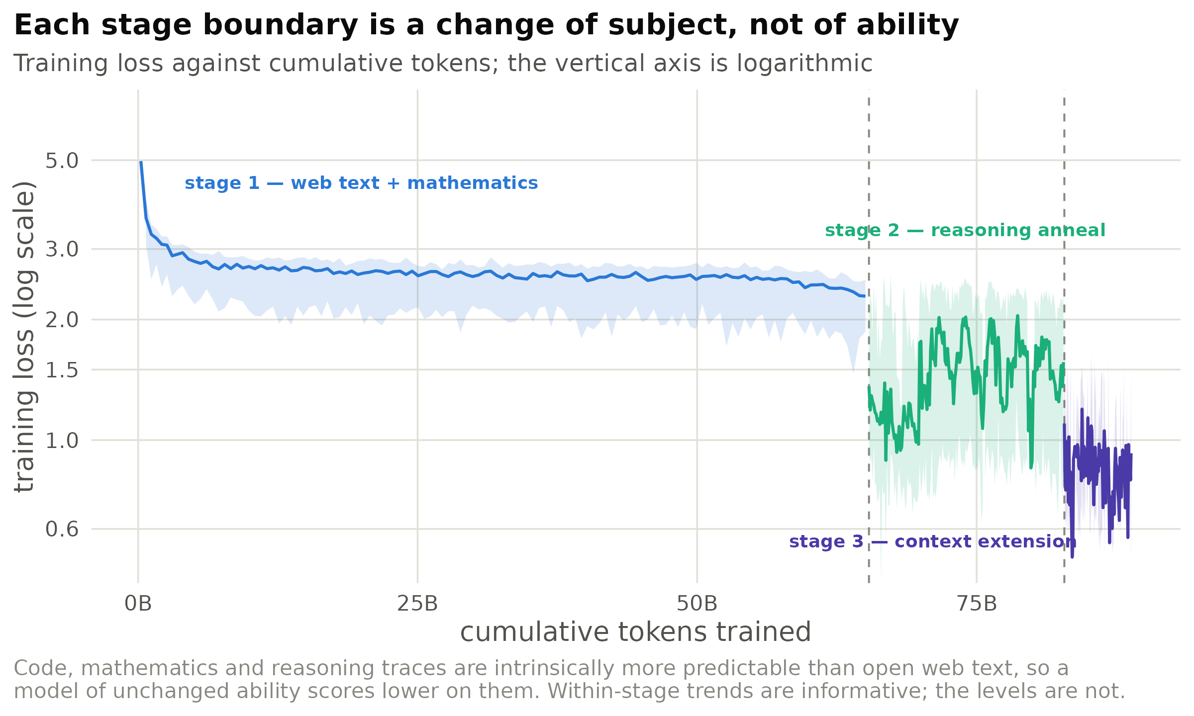
Figure 5: Median loss within each short window of the run; the band spans the 10th to 90th percentile inside the window, which is a measure of how much consecutive batches differ from one another.

The width of the band is itself a finding. A corpus that interleaves web text and mathematics produces batches of visibly different difficulty, so per-step loss is noisy by construction — anything from 1.7 to 3.2 was normal in stage 1, with the mathematics shards at the bottom of the range. No divergence occurred, and no non-finite loss was recorded at any point in the run.

Context that is trained, not extrapolated

Argonne 3.0 used rotary position embeddings with a large wavelength parameter (θ = 10⁶), which is often assumed to let a model generalise beyond the sequence length it was trained on. On this architecture it does not. Measured directly, by comparing the checkpoint that entered the context-extension stage against the weights it produced:

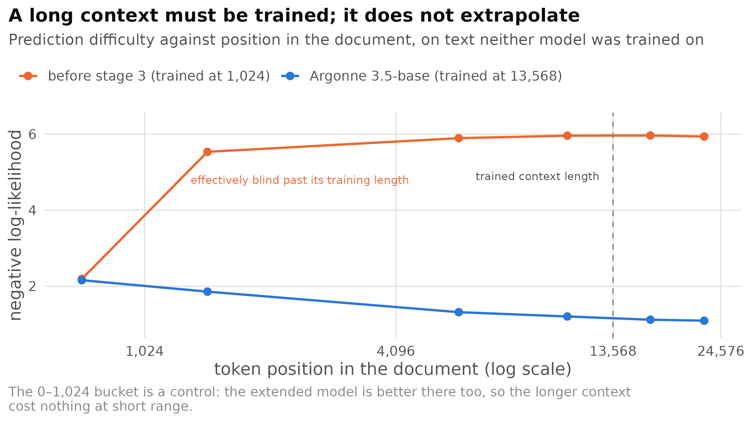
Figure 6: Held-out arXiv text, negative log-likelihood by token position; lower is better. The vertical dashed line marks the length the final stage actually trained on.

Three properties of this result matter. Before the final stage the model is coherent within its 1,024-token window and almost useless beyond it, with the break landing exactly at the pretraining length — extrapolation did not happen at all. After the stage, prediction improves monotonically with position and keeps improving past 13,568 tokens, which is the signature of a model that has learned to use distance rather than one that has merely been shown longer inputs. And the short-context control improved, so nothing was traded away; at an earlier point in the same stage that control had been slightly worse, and the terminal decay recovered it.

Eight-bit matrix multiplication

The one throughput change was to compute the large matrix multiplications in 8-bit floating point while keeping the master weights in 32-bit. A dedicated search measured this before it was adopted: an individual matrix multiplication runs about 1.83× faster, but only about 44% of a training step is spent in eligible operations, so the end-to-end gain is about 1.25× — at indistinguishable quality and with no non-finite values in any run. Two conditions were not optional. The scaling arithmetic must be fused into the multiplication by the compiler, since running it interpreted is roughly 2.3× slower than not using FP8 at all; and the vocabulary had to be padded from 151,669 to 151,680 so that the output projection was eligible too, which the export then trims back.

Two other candidate speedups were tested and rejected. Recomputing the loss in chunks to free memory made the run 25% slower at a context of 1,024, where the step is compute-bound rather than memory-bound. And the attention implementation, which the startup banner reported as a slow fallback, was measured at the real tensor shapes and found already to be running the fast kernel — the banner was a static string, not a runtime observation. Both investigations concluded that the configuration was already near-optimal, which is a useful thing to be able to establish.

The same audit turned up a finding that belongs here rather than in a footnote. The architecture includes an interleaved local-attention pattern, in which alternate layers attend only to a 256-token neighbourhood — one of the features the earlier article credited to Argonne 3.0. It has never actually run. The kernel that implements windowed attention is absent from the installed software, so the model silently falls back to full attention and the window is ignored, in every production run of both versions. Nothing was lost, because the recipe search measured local attention as quality-neutral at a context of 1,024 — but a documented architectural feature was inert for two model generations, and only a direct measurement at the tensor level revealed it.

What it actually takes to run for a month

The run occupied 108 scheduler allocations of two or three GPUs each, submitted as a self-resubmitting chain that saves a checkpoint and exits cleanly before each wall-clock limit.

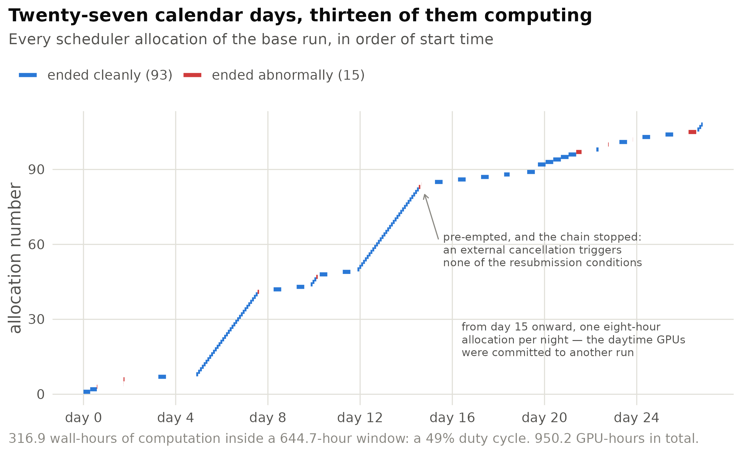
Figure 7: Each horizontal segment is one scheduler allocation. Horizontal gaps are queueing, deliberate pauses, and two chain failures. Colour marks how the allocation ended.

Half the elapsed time was not computation. Some of that is queueing on a shared machine and some was deliberate — the GPUs were lent to other work — but two stretches were failures of the chain itself, and both are worth recording because neither produced an error message.

The first is visible above. A slice was pre-empted by the scheduler, which delivers an external termination signal; the resubmission logic fires on clean exit, on its own wall-clock warning, and on a non-zero crash, and an external cancellation is none of those. The chain simply stopped, having lost no progress, with nothing queued and nothing logged. The second was a nightly placeholder job whose name collided with an unrelated interactive job of the same name, so it was cancelled by its own owner nineteen seconds after starting.

Two sizing lessons came out of the same run, both instances of measuring the wrong moment. Host memory was set from the observed steady state of 115 GiB, but the true peak is the resume transient, when all three processes load a 34 GB checkpoint simultaneously — about 146 GiB, which had been passing with four gigabytes to spare. Separately, a checkpoint-extraction job sized from a reported peak of 23.4 GB was killed at 27.0 GiB, because periodic sampling misses a short allocation spike. The reliable rule is to size such jobs from the checkpoint file, not from an observation.

One further operational rule was learned the hard way and is worth stating plainly: an automatic checkpoint-pruning policy, added to control disk use, deleted 14 of 17 checkpoints overnight. Whether old checkpoints are expendable is a judgement about which results are still needed, and it belongs to whoever owns the run rather than to a script.

Lessons from the base run

1. Hold the architecture fixed to learn something. Argonne 3.5 changed no component of Argonne 3.0, which is the only reason the recipe and data effects are attributable at all. The temptation in this kind of work is to redesign the model at the same time; resisting it turned a new version into an experiment.
2. Design the capability into pretraining instead of repairing it afterwards. Mixing mathematics into the corpus from the first step accomplished, at no measured cost to general knowledge, what a corrective stage plus a reconciling weight average had accomplished imperfectly before — and, as the companion article shows, it removed both stages from the pipeline that follows.
3. A default of zero is not a safe default. The single largest deficiency in the previous recipe was a parameter left unset, and it was invisible in every artefact a training run normally produces: the loss curve, the step count and the exported weights all looked exactly as expected.
4. Verify that a feature is running, not merely configured. A long-context parameter that was assumed to extrapolate did not; an attention pattern that was documented and configured never executed at all. Both took a direct measurement to establish, and neither would ever have appeared in a log.
5. Operational engineering decides whether a month-long run finishes. Half the elapsed time of this run was not computation, and the two chain failures, the memory mis-sizing and the over-eager pruning rule were each silent. None of it is interesting, and all of it is load-bearing.

What comes next

The base model is the expensive half of the work — 950 GPU-hours against the roughly 17 that turn it into something a person can talk to — but it is also the half that decides how good the finished model can be. The companion article takes this checkpoint through instruction tuning, preference tuning and chain-of-thought training; measures how much of the gain above survives into a deployable model; and describes the data defect that turned out to cost more than any of the choices made deliberately:

• Argonne 3.5-think: From Base Model to Reasoning Model

Availability

• Model: argonne-3.5-base on Hugging Face, alongside its Argonne 3.0 counterpart and the rest of the family.
• Code: github.com/PursuitOfDataScience/ArgonneAI — the complete training pipeline, one branch per version, together with the chronological training log from which every number above is drawn.
• Earlier articles in this series: Pretraining a Language Model From Scratch: Argonne 1.0 to 3.0 and How I Taught a Small Language Model to Reason.